
Correlation | CBSE Class 11 Economics Notes
On this page

This note covers the meaning and types of correlation, correlation and causation, scatter diagrams, Karl Pearson’s coefficient and its properties, calculation through deviations and transformed values, Spearman’s rank correlation, ranking procedures and repeated ranks.
What does correlation measure?
Definition: Correlation studies and measures the direction and intensity, or strength, of the relationship between variables. It measures covariation, meaning variation together, rather than causation, meaning a cause-and-effect relationship.
A variable is a characteristic whose value can change. Temperature, sales of ice-creams and the price of tomatoes are variables. Correlation analysis examines whether changes in one variable are associated with changes in another, and describes the nature of that association.
Which questions does correlation analysis answer?
- Is there a relationship between the two variables being studied?
- When the value of one changes, does the value of the other change?
- Do the variables move in the same direction or in opposite directions?
- How strong is the relationship between their movements?
The distinction between direction and intensity matters. Direction concerns whether values move together or oppositely. Intensity concerns how closely the movements are associated. Merely identifying the direction does not give a numerical measure of the strength of the relationship.
How do economic examples introduce the idea?
As summer heat rises, hill stations attract more visitors and ice-cream sales become brisk. Temperature is therefore related to visitor numbers and ice-cream sales. These examples introduce relationships involving changes in two variables rather than a description of just one variable.
In a local mandi, meaning a market, increasing supplies of tomatoes are associated with falling prices. When the local harvest reaches the market, the price falls from Rs 40 per kilogram to Rs 4 per kilogram or even less. Here, Rs denotes rupees.
Correlation analysis gives a systematic way of examining such relationships. It does not stop at noticing that values differ: it asks whether their movements have a definite association. A complete interpretation must consider both the direction and the strength of that association.
Why does correlation not establish causation?
Correlation does not imply causation. A relationship between two variables does not by itself show that a change in one causes the change in the other. Some relationships admit a cause-and-effect interpretation, while others may be coincidence or reflect another variable’s influence.
How can relationships arise?
Movements in a commodity’s price and quantity demanded form part of demand theory. Low agricultural productivity is related to low rainfall. Such relationships may be given a cause-and-effect interpretation, but the presence of correlation alone is not the justification for doing so.
The arrival of migratory birds in a sanctuary and birth rates in the locality cannot be given a cause-and-effect interpretation. The relationship is a simple coincidence. Shoe size and money in a person’s pocket provide another example of a relationship that is difficult to explain.
A third variable is another factor affecting both variables under consideration. Its influence may create a relationship between them even when neither variable is causing the other to change. The ice-cream and drowning example illustrates why this possibility matters.
What does the ice-cream example show?
Higher temperatures lead to brisk ice-cream sales. More people also start visiting swimming pools to escape the heat. This might have raised the number of deaths by drowning. The victims are not drowned because they ate ice-creams; temperature lies behind the association.
Note: The association between ice-cream sales and drowning deaths must not be read as evidence that eating ice-creams causes drowning. Examine the circumstances and the possible influence of temperature.
Context also matters when doctors are sent to villages affected by an epidemic. A positive association between doctors sent and deaths does not establish that doctors caused deaths. Many reported deaths could be terminal cases, while the benefit of medical care becomes visible only after some time.
It is also possible that reported deaths are not due to the epidemic. Understanding the time period and the circumstances is therefore necessary before interpreting a calculated coefficient. Statistical methods are no substitute for common sense.
How do positive, negative and linear relationships differ?
Positive correlation occurs when variables move in the same direction. Income and consumption illustrate this: rising income accompanies rising consumption, while falling income accompanies falling consumption. Temperature and ice-cream sales also move in the same direction.
Negative correlation occurs when variables move in opposite directions. A fall in the price of apples accompanies an increase in demand; a rise in price accompanies a decrease in demand. The negative sign describes direction, rather than an absence of relationship.
Which examples distinguish the directions?
| Variables | Associated movement | Direction |
|---|---|---|
| Income and consumption | Both rise or both fall | Positive |
| Temperature and ice-cream sales | Sales become brisk as temperature rises | Positive |
| Price of apples and demand | Demand increases when price falls | Negative |
| Interest rate and demand for funds | Demand for funds falls as interest rises | Negative |
| Study time and chances of failing | Chances of failing decline with more study time | Negative |
A linear relationship is one that can be represented by a straight line. A non-linear relationship follows a pattern that is not a straight line. An upward or downward movement need not, by itself, establish that the pattern is linear.
Which techniques study these relationships?
A scatter diagram presents the association visually without supplying a specific numerical value. Karl Pearson’s coefficient of correlation gives a numerical measure of a linear relationship between two variables. Spearman’s rank correlation measures linear association between the ranks assigned to items.
A rank is an item’s position in an ordering. An attribute, such as honesty or physical appearance, cannot be measured numerically in the same way as income or height. Ranking provides a way of studying association when precise numerical measurement is unavailable.
These techniques therefore answer related questions in different ways. A visual examination shows the form of the relationship. A coefficient gives a numerical measure, but its interpretation depends on the kind of data and the kind of relationship being measured.
How should a scatter diagram be drawn and interpreted?
A scatter diagram represents corresponding observations as points on graph paper. Let X denote the first variable and Y the second. Each point shows one observed value of X paired with the corresponding observed value of Y.
What steps organise the visual examination?
- Identify the paired observations of the two variables being studied.
- Plot each pair as a point using the X and Y axes.
- Examine whether the points form an upward, downward or directionless pattern.
- Examine their closeness to a line and whether the pattern is straight or curved.
The closeness of the points and their overall direction indicate the relationship. Points widely dispersed around a line suggest low correlation. Points close to a straight line indicate a linear association; when all points lie on the line, the correlation is perfect.
What the figure shows
Positive correlation
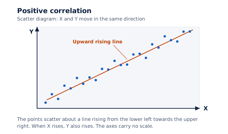
The horizontal axis is X and the vertical axis is Y. Points lie around a straight line rising from the lower left towards the upper right.
Drawn by One Young India. See Fig. 6.1 in your NCERT textbook
What the figure shows
Negative correlation
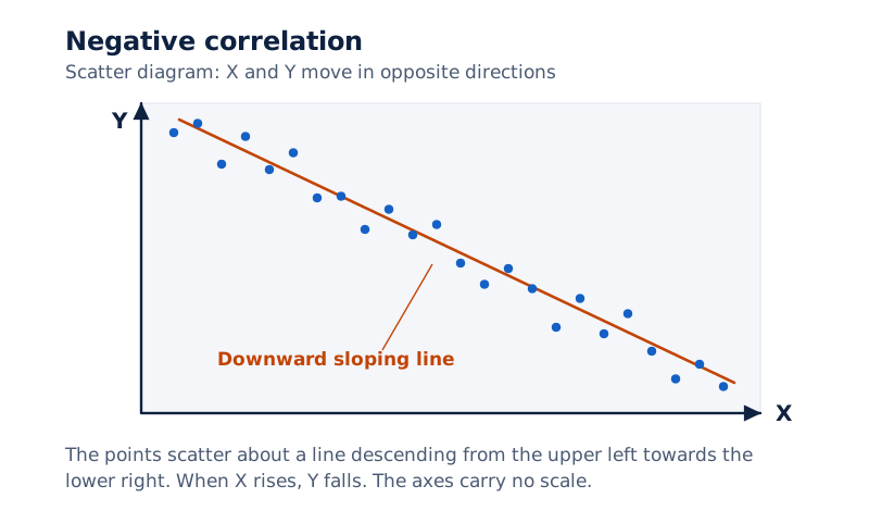
The axes are labelled X and Y. Points lie around a straight line descending from the upper left towards the lower right.
Drawn by One Young India. See Fig. 6.2 in your NCERT textbook
How do the other patterns differ?
What the figure shows
No correlation
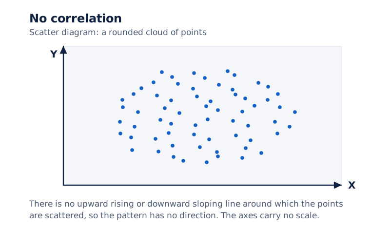
A roughly rounded cloud of points appears between the X and Y axes. There is no upward or downward sloping line around which the points are arranged.
Drawn by One Young India. See Fig. 6.3 in your NCERT textbook
What the figure shows
Perfect correlation
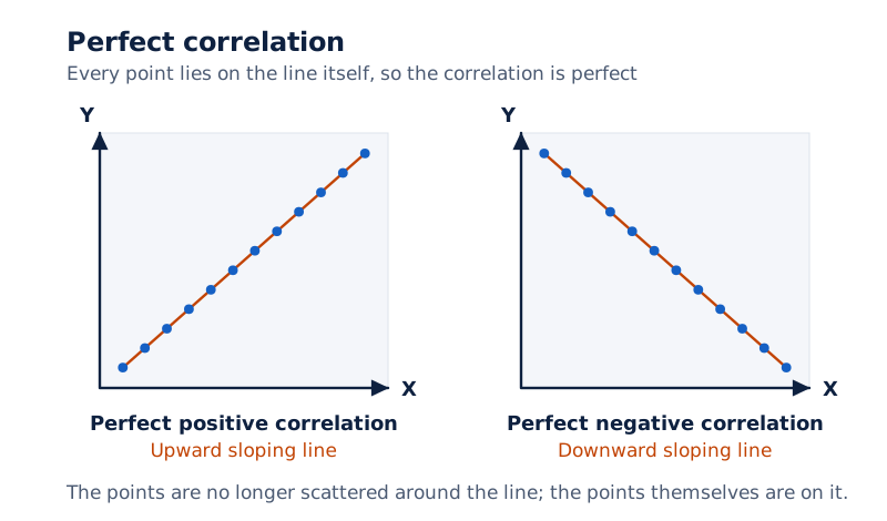
Figure 6.4 places points on an upward sloping straight line. Figure 6.5 places points on a downward sloping straight line.
Drawn by One Young India. See Figs. 6.4 and 6.5 in your NCERT textbook
What the figure shows
Non-linear relationships
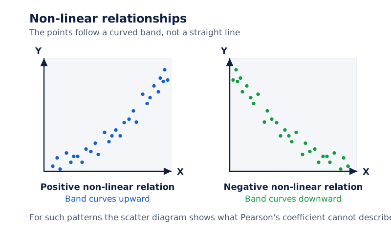
Figure 6.6 shows an upward curved band of points. Figure 6.7 shows a downward curved band of points. Both have X and Y axes.
Drawn by One Young India. See Figs. 6.6 and 6.7 in your NCERT textbook
Inspect the scatter diagram first before calculating Pearson’s coefficient. For a non-linear relationship, that coefficient can be misleading. The scatter diagram is not confined to linear relations, so it can reveal a pattern that a numerical measure of linear correlation does not adequately describe.
What formulas define Karl Pearson’s correlation coefficient?
Pearson’s coefficient, written r, is also called the product moment correlation coefficient or simple correlation coefficient. It gives a precise numerical measure of the direction and degree of linear relationship between X and Y.
What do the symbols mean?
Let N be the number of paired observations and Σ mean the sum over all observations. The symbols X̄ and Ȳ denote the arithmetic means, found by dividing the sum of each variable’s values by N.
X̄ = ΣX / N
Ȳ = ΣY / N
A deviation is the difference between a value and its mean. Define x = X − X̄ and y = Y − Ȳ. The lower-case symbols x and y therefore denote deviations, rather than the original observations X and Y.
Variance is the mean of the squared deviations. Let σₓ² and σᵧ² denote the variances of X and Y. Their positive square roots, σₓ and σᵧ, are the corresponding standard deviations, which measure dispersion around the means.
σₓ² = Σx² / N
σᵧ² = Σy² / N
The superscript ² means squaring. Covariance, written Cov(X,Y), is the mean product of the paired deviations. The product xy multiplies x by its corresponding y; it does not pair values from different observations.
Cov(X,Y) = Σxy / N
How are the equivalent formulas used?
r = Cov(X,Y) / (σₓσᵧ)
r = Σxy / √(Σx² × Σy²)
Here √ means the positive square root and × means multiplication. The second expression calculates the same coefficient directly from the deviation products and the two sums of squared deviations.
r = [NΣXY − (ΣX)(ΣY)] / √([NΣX² − (ΣX)²][NΣY² − (ΣY)²])
This last form uses original values. ΣXY means the sum of paired products; ΣX² means the sum of squared X values; (ΣX)² means the square of their sum. These last two expressions must be kept distinct.
Because the standard deviations in the denominator are positive, the sign of covariance determines the sign of r. Zero covariance gives zero correlation. The formulas provide alternative routes to the same measure; the available data and the amount of arithmetic guide the choice.
What are the properties and limitations of Pearson’s coefficient?
r is a pure number without a unit. The units used for the original observations are not attached to the coefficient. For example, a correlation between height in feet and weight in kilograms could be 0.7, with neither feet nor kilograms attached.
How do sign and magnitude guide interpretation?
| Value or feature | Interpretation |
|---|---|
| Positive r | The variables move in the same direction |
| Negative r | The variables move in opposite directions |
| r = 1 | Perfect positive linear correlation |
| r = −1 | Perfect negative linear correlation |
| r = 0 | No linear relationship; another type of relationship may exist |
| r close to +1 or −1 | Strong linear relationship |
| r close to zero | Weak linear relationship; a non-linear relationship may exist |
The permitted range is −1 ≤ r ≤ 1, where ≤ means “less than or equal to”. A result outside this range indicates an error in calculation. A negative coefficient close to −1 represents strong negative correlation, rather than weak correlation.
For marks in English and Statistics, a coefficient of 0.1 indicates positive but weak correlation. Students with high English marks may obtain relatively low Statistics marks. The sign identifies the direction; proximity to zero identifies the weakness of the linear association.
What do changes of origin and scale mean?
A change of origin subtracts a chosen constant, while a change of scale divides by a common factor. Define transformed variables U and V by U = (X − A)/B and V = (Y − C)/D.
Here A and C are assumed means, meaning convenient values chosen as reference points. B and D are common factors of the same sign. Under this transformation, r between U and V equals r between X and Y.
Note: Zero correlation means no linear relationship. It does not establish statistical independence, meaning that knowing one variable gives no information about the other, because another form of relationship may be present.
Pearson’s coefficient should be used only for a linear relationship. Its numerical precision does not remove this limitation or establish causation. Interpretation must therefore combine the coefficient with the scatter pattern and an understanding of the observations.
How is Pearson’s coefficient calculated from mean deviations?
The method using deviations from actual means begins with paired observations, calculates each variable’s mean and then uses deviations from those means. Keeping each observation’s two values together is essential because the numerator uses products of corresponding deviations.
Worked example 1. Calculate the correlation between farmers’ years of schooling, X, and annual yield per acre in thousands of rupees, Y. The paired values are (0,4), (2,4), (4,6), (6,10), (8,10), (10,8) and (12,7).
Answer: N = 7, ΣX = 42 and ΣY = 49, so X̄ = 6 and Ȳ = 7. With Σxy = 42, Σx² = 112 and Σy² = 38, r = 42/√(112 × 38) = 0.644.
How is the calculation table prepared?
For these observations, x = X − 6 and y = Y − 7. The columns x² and y² contain the squares of those deviations, while xy contains their paired products. The table preserves the observations and calculated entries together.
| X: schooling years | x | x² | Y: yield in thousands of rupees | y | y² | xy |
|---|---|---|---|---|---|---|
| 0 | −6 | 36 | 4 | −3 | 9 | 18 |
| 2 | −4 | 16 | 4 | −3 | 9 | 12 |
| 4 | −2 | 4 | 6 | −1 | 1 | 2 |
| 6 | 0 | 0 | 10 | 3 | 9 | 0 |
| 8 | 2 | 4 | 10 | 3 | 9 | 6 |
| 10 | 4 | 16 | 8 | 1 | 1 | 4 |
| 12 | 6 | 36 | 7 | 0 | 0 | 0 |
The column totals required are ΣX = 42, Σx² = 112, ΣY = 49, Σy² = 38 and Σxy = 42. The coefficient is positive, and its value is also large. Schooling and annual yield are positively associated in these observations.
What sequence keeps the working clear?
- Count the paired observations and calculate the two arithmetic means.
- Subtract the appropriate mean from each original value to obtain deviations.
- Calculate each squared deviation and each product of corresponding deviations.
- Add the required columns, substitute in the formula and interpret the result.
The standard-deviation form gives the same answer. Here σₓ = √(112/7), σᵧ = √(38/7) and covariance is 42/7. Dividing covariance by the product of the standard deviations again gives 0.644.
The association underlines the importance of farmers’ education. Its interpretation must still retain the distinction between covariation and causation: the calculated coefficient describes the relationship in the paired data and does not itself prove a cause-and-effect explanation.
How does the step-deviation method simplify calculation?
The step-deviation method reduces the burden of arithmetic when original observations are large. It transforms the values by subtracting convenient constants and dividing by common factors. The coefficient remains unchanged under the same-sign scale transformation described earlier.
Which data and transformations are used?
Worked example 2. Find correlation for price index X = 120, 150, 190, 220, 230 and money supply Y = 1800, 2000, 2500, 2700, 3000, in Rs crores. A price index measures changes in prices; money supply is the quantity of money, and a crore is ten million.
Answer: Use U = (X − 100)/10 and V = (Y − 1700)/100. Then ΣU = 41, ΣV = 35, ΣU² = 423, ΣV² = 343 and ΣUV = 378. Substitution gives r = 0.98, indicating strong positive correlation.
Here U and V are the transformed observations. The constants 100 and 1700 provide the reference points. Divisors 10 and 100 are both positive, meeting the condition that the scale factors have the same sign.
| U | V | U² | V² | UV |
|---|---|---|---|---|
| 2 | 1 | 4 | 1 | 2 |
| 5 | 3 | 25 | 9 | 15 |
| 9 | 8 | 81 | 64 | 72 |
| 12 | 10 | 144 | 100 | 120 |
| 13 | 13 | 169 | 169 | 169 |
How are transformed values substituted?
r = [ΣUV − (ΣU)(ΣV)/N] / √([ΣU² − (ΣU)²/N][ΣV² − (ΣV)²/N])
With N = 5, the substitution is r = [378 − (41 × 35)/5] / √([423 − 41²/5][343 − 35²/5]) = 0.98. The symbols have the same summation meaning as before, now applied to transformed values.
The result indicates a strong positive relationship between the price index and money supply. As money supply grows, the price index also rises. This association is an important premise of monetary policy, meaning policy concerned with money supply.
U and V are not deviations from the actual arithmetic means. Therefore, use the formula that retains the correction involving their sums. The simplification changes the numbers used in the arithmetic, while the resulting coefficient describes the original pair of variables.
When is Spearman’s rank correlation useful?
Spearman’s rank correlation coefficient was developed by the British psychologist C. E. Spearman. It measures the linear association between ranks assigned to items, rather than between the original numerical values of those items.
Which situations favour ranks?
- Height and weight may be ranked when measuring rods and weighing machines are unavailable.
- Fairness, honesty and beauty cannot be measured in the same way as income, weight or height.
- Rank correlation can be used in some cases where a relationship has a clear direction but is non-linear.
- Extreme values do not affect Spearman’s coefficient, which can be very useful when such values occur.
Extreme values are observations far from the other values. Rank correlation uses their positions in an ordering rather than the size of their numerical distance from other observations. In this respect, it is better than Pearson’s coefficient.
For attributes such as beauty, measurement is at most relative. Some people would argue that even ranking is not possible because standards and criteria may differ between people and cultures. Ranking should not be presented as an unquestionable objective measurement.
What formula applies when ranks are not repeated?
Write rₛ for Spearman’s coefficient, n for the number of paired observations and D for the difference between the two ranks of the same item. Then D² is its squared rank difference and ΣD² is the sum of these squares.
rₛ = 1 − 6ΣD² / (n³ − n)
The superscript ³ means cubing. Like Pearson’s coefficient, rₛ lies between −1 and +1 and is interpreted through its sign and strength. The data may supply ranks directly, require ranks to be assigned, or contain repeated ranks needing special treatment.
Rank correlation is generally not as accurate as the ordinary method because it does not use all the information in the numerical data. A first difference is the difference between consecutive values arranged in order of magnitude.
Such first differences are almost never constant. Data usually cluster around central values with smaller differences in the middle of the array. If first differences were constant, the ordinary and rank coefficients would give identical results.
How is rank correlation calculated from supplied ranks or marks?
When ranks are already supplied, compare the two ranks assigned to each item. When only original values are supplied, first construct a ranking for each variable. In both cases, preserve the correspondence between observations before calculating rank differences.
What happens when judges supply the ranks?
Worked example 3. For five competitors in a beauty contest, judge A assigns ranks 1, 2, 3, 4, 5 and judge B assigns ranks 2, 4, 1, 5, 3. Find their rank correlation.
Answer: Taking each rank of A minus the corresponding rank of B gives D = −1, −2, 2, −1, 2. Thus ΣD² = 14 and rₛ = 1 − (6 × 14)/(5³ − 5) = 0.3.
| Rank assigned by A | Rank assigned by B | D | D² |
|---|---|---|---|
| 1 | 2 | −1 | 1 |
| 2 | 4 | −2 | 4 |
| 3 | 1 | 2 | 4 |
| 4 | 5 | −1 | 1 |
| 5 | 3 | 2 | 4 |
The sum of squared differences is 14. A positive coefficient indicates positive association between the rankings. The method compares how the judges order the same competitors, rather than measuring beauty in numerical units.
How are ranks assigned when marks are given?
Worked example 4. Students A, B, C, D and E score 85, 60, 55, 65 and 75 per cent in Statistics, and 60, 48, 49, 50 and 55 per cent in Economics, respectively. Find their rank correlation.
Answer: Giving the highest mark rank 1, Statistics ranks are 1, 4, 5, 3, 2 and Economics ranks are 1, 5, 4, 3, 2. Their differences are 0, −1, 1, 0, 0. Hence ΣD² = 2 and rₛ = 1 − (6 × 2)/(5³ − 5) = 0.9.
Here % means per cent, or out of a hundred.
| Student | Statistics marks (%) | Economics marks (%) | Statistics rank | Economics rank |
|---|---|---|---|---|
| A | 85 | 60 | 1 | 1 |
| B | 60 | 48 | 4 | 5 |
| C | 55 | 49 | 5 | 4 |
| D | 65 | 50 | 3 | 3 |
| E | 75 | 55 | 2 | 2 |
Once the rankings have been assigned, the original marks are replaced by their ranks in the calculation. The resulting 0.9 describes strong positive association between the students’ rankings in the two subjects.
How should repeated ranks be handled?
Repeated ranks arise when two or more observations have the same value. These observations receive a common rank equal to the mean of the positions they would have occupied if their values had been slightly different.
How are average ranks allocated?
Consider the paired observations in the table below. The X values are all different, but some Y values repeat. Ranking the largest value first places the three occurrences of Y = 50 in positions 9, 10 and 11.
Each of those three observations receives average rank 10. The following observation receives the next rank after the positions already occupied, rather than the rank immediately after the average. This keeps the ranking consistent with the number of observations.
| X | Y | Rank of X | Rank of Y | D | D² |
|---|---|---|---|---|---|
| 1200 | 75 | 1 | 5.5 | −4.5 | 20.25 |
| 1150 | 65 | 2 | 7 | −5 | 25.00 |
| 1000 | 50 | 3 | 10 | −7 | 49.00 |
| 990 | 100 | 4 | 1 | 3 | 9.00 |
| 800 | 90 | 5 | 2.5 | 2.5 | 6.25 |
| 780 | 85 | 6 | 4 | 2 | 4.00 |
| 760 | 90 | 7 | 2.5 | 4.5 | 20.25 |
| 750 | 40 | 8 | 12 | −4 | 16.00 |
| 730 | 50 | 9 | 10 | −1 | 1.00 |
| 700 | 60 | 10 | 8 | 2 | 4.00 |
| 620 | 50 | 11 | 10 | 1 | 1.00 |
| 600 | 75 | 12 | 5.5 | 6.5 | 42.25 |
The sum for the D² column is 198.00. Equal observations must receive the same average rank; assigning them different consecutive ranks would incorrectly distinguish equal values.
What correction does the formula require?
A correction factor is the additional term used for a group of tied ranks. Let m be the number of observations in that tied group. Its correction is (m³ − m)/12.
For successive tied groups, write their sizes as m₁, m₂, …, where the subscripts label the groups and the dots indicate further groups. The repeated-rank expression is:
rₛ = 1 − 6[ΣD² + (m₁³ − m₁)/12 + (m₂³ − m₂)/12 + …] / [n(n² − 1)]
- Arrange the values in rank order for each variable.
- Give each tied group the average of the positions it occupies.
- Calculate paired rank differences, square them and find their sum.
- Include the correction factors for tied groups before applying the repeated-rank formula.
The essential distinction is between allocating average ranks and including corrections. Both belong to the repeated-rank procedure. Averaging the ranks does not remove the need to consider the additional terms in the formula.
Glossary
- Correlation — A statistical study of the direction and intensity of association between variables.
- Covariation — Variation together, where changes in one variable are associated with changes in another.
- Causation — A cause-and-effect relationship, which the presence of correlation alone does not establish.
- Positive correlation — Association in which the two variables move together in the same direction.
- Negative correlation — Association in which movement in one variable accompanies opposite movement in another.
- Linear relationship — A relationship whose pattern can be represented by a straight line.
- Scatter diagram — A graph of paired observations that visually displays the form of their relationship.
- Pearson’s coefficient — A unit-free numerical measure of the direction and degree of linear relationship.
- Covariance — The mean product of corresponding deviations of two variables from their arithmetic means.
- Standard deviation — The positive square root of variance, measuring dispersion around the arithmetic mean.
- Step deviation — Transformation by subtracting reference values and dividing by factors to simplify correlation calculations.
- Rank correlation — A measure of linear association between the ranks assigned to corresponding items.
- First difference — The difference between consecutive values in a series arranged in order of magnitude.
- Repeated ranks — Ranks allocated to equal observations using the average of their occupied positions.
Common errors and misconceptions
- Misconception: Correlation proves that one variable causes the other. Correct: It measures covariation. Coincidence or a third variable may explain an association, so a cause-and-effect conclusion does not follow from correlation alone.
- Misconception: A negative coefficient indicates a weak relationship. Correct: Its sign indicates opposite movement. A coefficient close to −1 represents strong negative linear correlation; closeness to zero indicates weak linear correlation.
- Misconception: Zero correlation means the variables are independent. Correct: It means there is no linear relationship. A different form of relationship may still exist and may be visible in a scatter diagram.
- Misconception: Pearson’s coefficient can describe every relationship adequately. Correct: It measures linear association. For a non-linear relationship, calculating it can be misleading, so examine the scatter diagram first.
- Misconception: Correlation between height and weight has a combined height-and-weight unit. Correct: The coefficient is a pure number. The units of the original variables do not become units of r.
- Misconception: ΣX² and (ΣX)² are interchangeable. Correct: The first adds squared observations; the second squares the sum of observations. The original-value formula contains both and distinguishes their roles.
- Misconception: Equal values can receive different ranks, with no adjustment. Correct: Give equal values the average of their occupied ranks and use the correction terms required by the repeated-rank formula.
Exam-style questions with model answers
Q1. Define correlation and state whether it establishes causation. [2 marks]
- Correlation studies and measures the direction and intensity of the relationship between variables.
- It measures covariation, not causation; a relationship between variables does not itself establish cause and effect.
Q2. Interpret Pearson’s coefficients of +1, −1 and 0, distinguishing the conclusion at zero from independence. [3 marks]
- A coefficient of +1 means perfect positive correlation: the variables have an exact linear relationship and move in the same direction.
- A coefficient of −1 means perfect negative correlation: the variables have an exact linear relationship but move in opposite directions.
- A coefficient of 0 means no linear relationship. It does not establish independence, because another type of relationship may still be present.
Q3. Explain four reasons for using Spearman’s rank correlation. [4 marks]
- It can be used when precise measurement is unavailable, as when students’ heights and weights can be ranked but measuring equipment is absent.
- It can study attributes such as honesty or fairness, which cannot be measured in the same way as income or weight.
- It can be used in some cases where the relationship has a clear direction but is non-linear.
- It is not affected by extreme values. In this respect, it is better than Pearson’s coefficient and can be very useful for such data.
Q4. Farmers’ schooling years are 0, 2, 4, 6, 8, 10, 12; corresponding annual yields per acre in thousands of rupees are 4, 4, 6, 10, 10, 8, 7. Calculate Pearson’s coefficient and interpret it. [5 marks]
- Let X denote schooling years, Y annual yield and N the number of pairs. Here N = 7, ΣX = 42 and ΣY = 49, giving means X̄ = 6 and Ȳ = 7.
- Subtracting the respective means gives x = −6, −4, −2, 0, 2, 4, 6 and y = −3, −3, −1, 3, 3, 1, 0.
- Squaring the deviations and adding gives Σx² = 112 and Σy² = 38. Multiplying corresponding deviations and adding gives Σxy = 42.
- Apply r = Σxy/√(Σx² × Σy²). Substitution gives r = 42/√(112 × 38) = 0.644.
- The association between schooling and yield is positive and the value is large. The coefficient describes covariation and does not itself prove causation.
Q5. Price index values are 120, 150, 190, 220, 230; corresponding money supply values in Rs crores are 1800, 2000, 2500, 2700, 3000. Use U = (X − 100)/10 and V = (Y − 1700)/100, where X is price index and Y is money supply, to calculate correlation. [5 marks]
- The transformations subtract fixed reference values and divide by positive factors. These factors have the same sign, so the correlation between U and V equals that between the original variables.
- The transformed observations are U = 2, 5, 9, 12, 13 and V = 1, 3, 8, 10, 13. There are five corresponding pairs, so N = 5.
- Adding the values, their squares and their paired products gives ΣU = 41, ΣV = 35, ΣU² = 423, ΣV² = 343 and ΣUV = 378.
- Substitute in the original-value formula: r = [378 − (41 × 35)/5]/√([423 − 41²/5][343 − 35²/5]) = 0.98.
- The result indicates strong positive correlation between the price index and money supply. Their observed movements are in the same direction.
Q6. Judge A gives five competitors ranks 1, 2, 3, 4, 5; judge B gives the same competitors ranks 2, 4, 1, 5, 3. Calculate Spearman’s coefficient. [3 marks]
- Let D be A’s rank minus B’s rank for the same competitor. The paired differences are −1, −2, 2, −1 and 2.
- The squared differences are 1, 4, 4, 1 and 4, giving ΣD² = 14. There are five competitors, so n = 5.
- Substitute in rₛ = 1 − 6ΣD²/(n³ − n): rₛ = 1 − 84/120 = 0.3. The rankings have positive correlation.
Q7. Students A, B, C, D, E obtain Statistics percentages 85, 60, 55, 65, 75 and Economics percentages 60, 48, 49, 50, 55 respectively. Assign highest marks rank 1 and calculate rank correlation. [4 marks]
- In student order, the Statistics ranks are 1, 4, 5, 3, 2, while the Economics ranks are 1, 5, 4, 3, 2.
- Subtracting corresponding Economics ranks from Statistics ranks gives differences D = 0, −1, 1, 0, 0.
- Squaring and adding gives ΣD² = 2. With n = 5 students, the denominator n³ − n is 125 − 5 = 120.
- Thus rₛ = 1 − (6 × 2)/120 = 0.9. There is strong positive association between the students’ rankings in the two subjects.
Q8. Three equal observations occupy rank positions 9, 10 and 11. Explain their common rank, the next rank, and the correction factor for this group. [3 marks]
- Each tied observation receives the average of the occupied positions: (9 + 10 + 11)/3 = 10. Giving different ranks would wrongly distinguish equal observations.
- The next observation receives rank 12, because the tied group occupies positions through 11, despite each member being labelled with average rank 10.
- The group has m = 3 observations. Its correction factor is (m³ − m)/12 = (27 − 3)/12 = 2, added in the repeated-rank expression.
Key takeaways
- Correlation measures the direction and intensity of association between variables; its presence does not establish a cause-and-effect relationship.
- Positive correlation means movement in the same direction; negative correlation means movement in opposite directions.
- Scatter diagrams reveal the form of a relationship visually and should be examined before calculating Pearson’s coefficient.
- Pearson’s coefficient is unit-free and lies between −1 and +1; closeness to either endpoint indicates strong linear association.
- Zero correlation means no linear relationship, while a different form of relationship may still exist.
- Transforming observations by suitable changes of origin and scale simplifies calculations without changing the correlation coefficient.
- Spearman’s coefficient uses ranks and is useful when precise measurements are unavailable or some data contain extreme values.
- Equal observations receive average ranks, and the repeated-rank formula includes correction factors for the tied groups.
Test yourself
Why does a positive correlation between ice-cream sales and drowning deaths not prove causation?
Temperature influences ice-cream sales and swimming activity. More swimming might raise drowning deaths, without ice-cream consumption causing them.
What distinguishes perfect correlation from points scattered close to a straight line?
With perfect correlation, all points lie on the straight line; they are not merely scattered close to it.
What unit belongs to a correlation coefficient calculated from height in feet and weight in kilograms?
No unit belongs to the coefficient. It is a pure number regardless of the original measurement units.
What does a coefficient close to zero tell you?
It indicates weak linear association, but a non-linear relationship may still exist between the variables.
How does ΣX² differ from (ΣX)²?
ΣX² adds the squared observations, while (ΣX)² squares the sum of the observations.
Why are step deviations useful for large observations?
They replace large observations with simpler transformed values while preserving correlation under the stated same-sign scale condition.
Why is rank correlation generally less accurate than the ordinary method?
It replaces numerical values with ranks, so all the information concerning the original data is not utilised.
What rank is assigned to each of three equal values occupying positions 9, 10 and 11?
Each receives rank 10, the average of the three positions that the tied values occupy.
Write about it
Turn a question from this chapter into a paper.
The Writing Studio has a structure guide, a rubric and citation tools for 15 formats, from essays to research papers. Drafting is free with an account. Learnacy Essential adds feedback from an AI writing coach and submission to The OYI Review.
Learnacy Essential is ₹1,499 for the year. Publication depends on review and is not guaranteed.