
Measures of Central Tendency | CBSE Class 11 Economics Notes
On this page
This note covers central tendency, arithmetic mean, direct and short-cut methods, weighted mean, median, cumulative frequency, quartiles, percentiles, mode, and the choice of an appropriate average.
What does a measure of central tendency tell us?
Definition: A measure of central tendency summarises a collection of observations through a single typical or representative value. An observation is an individual value in the data being studied.
A long list of marks, incomes or land holdings contains information about individuals. An average provides a numerical summary of that list. Average rainfall, factory production and family income are examples of using one value to describe a larger collection.
Why can the same data require different averages?
Baiju is a farmer with 1 acre of land in Balapur, a village in Buxar district of Bihar. The village has 50 small farmers. Comparing his land with their holdings requires a summary of the whole set of holdings.
However, the question being asked matters. Is his holding above the ordinary average? Is it larger than what half the farmers own? Or is it larger than the holding size that occurs most frequently? These comparisons lead to different averages.
| Measure | Basis of the comparison |
|---|---|
| Arithmetic mean | Total value divided by the number of observations |
| Median | The middle position after arranging observations by size |
| Mode | The value occurring most frequently |
The arithmetic mean, median and mode are the three most commonly used averages. Geometric mean and harmonic mean are other types of average suitable in certain situations. The calculations here concern the three commonly used measures.
A representative value helps explain data briefly, but an average alone is not enough to compare series. Selecting a measure requires attention to both the purpose of the analysis and the nature of the distribution, meaning the way observations are spread across values.
How is arithmetic mean calculated for ungrouped data?
Ungrouped data lists observations individually. Its arithmetic mean is the sum of all the observed values divided by their number. The mean is usually written as X̄, read as “X bar”. Let X represent an observed value and N the total number of observations.
The symbol Σ, called sigma, means summation, or adding the specified values. Thus ΣX means the sum of all observations. The direct-method formula is Mean = ΣX / N. The word “Mean” in these formulas represents X̄.
What are the steps in the direct method?
- Identify all observations in the series.
- Add their values to obtain ΣX.
- Count the observations to obtain N.
- Divide the total by N and interpret the answer in the original unit.
Worked example 1. Calculate the mean of the economics test marks 40, 50, 55, 78 and 58.
Answer: Mean = (40 + 50 + 55 + 78 + 58) / 5 = 56.2 marks. This is the average mark of the five students in the economics test.
The calculation uses every student's mark. The number of observations is the number of students whose marks have been supplied, rather than the number of different marks that might appear in a longer list.
What does a mean represent?
The mean provides one summary value for the group. It is not a statement that every member has that value. In the test example, 56.2 describes the group's average even though it is not one of the five listed marks.
The direct method is straightforward, but adding many large numerical values can make the work lengthy. The assumed mean and step deviation methods simplify that arithmetic while calculating the same measure of central tendency.
How do assumed mean and step deviation simplify calculations?
An assumed mean is a value chosen as a starting point for calculation. Write it as A. A deviation is the signed difference between an observation and this starting value: d = X − A.
Add these differences, divide their sum by N, and add the result to A. The formula is Mean = A + Σd / N. A negative deviation belongs to an observation below A; a positive deviation belongs to an observation above A.
How should the starting value be chosen?
Any value can serve as A, whether or not it appears in the data. A centrally located value can simplify calculations. Choosing A does not mean assuming that it is the final answer: the average deviation provides the required correction.
Worked example 2. Ten families have weekly incomes, in rupees (Rs), of 850, 700, 100, 750, 5000, 80, 420, 2500, 400 and 360. Find their mean using A = 850.
Answer: The deviations are 0, −150, −750, −100, +4150, −770, −430, +1650, −450 and −490. Their sum is +2660. Mean = 850 + 2660 / 10 = Rs 1,116 per week.
What does step deviation add?
In the step deviation method, divide each deviation by a common factor, c. Write the reduced deviation as d′, read as “d prime”. Thus d′ = (X − A) / c. The common factor reduces the size of the numbers being handled.
The final formula is Mean = A + (Σd′ / N) × c. Multiplication by c restores the scale before the correction is added to the assumed mean. Forgetting this multiplication changes the answer.
For the same family incomes, take c = 10. The reduced deviations total 266. The calculation becomes 850 + (266 / 10) × 10 = Rs 1,116. Direct addition also gives a total income of Rs 11,160 and the same mean.
How is the mean calculated for a discrete frequency series?
A discrete frequency series records distinct values together with the number of times each occurs. This number is its frequency, written as f. Instead of writing a repeated value many times, multiply it by its frequency.
Here fX means frequency multiplied by the corresponding value. ΣfX is the sum of those products, and Σf is the total frequency. The direct-method formula is Mean = ΣfX / Σf. The denominator counts all observations represented in the table.
How do plot sizes illustrate the calculation?
The following housing-colony data has three plot sizes. The larger number of small plots must influence the mean. Giving each size equal importance would ignore how many plots actually belong to each category.
| Plot size X, square metres | Number of plots f | Product fX |
|---|---|---|
| 100 | 200 | 20000 |
| 200 | 50 | 10000 |
| 300 | 10 | 3000 |
| Total | 260 | 33000 |
Worked example 3. A colony has 200 plots of 100 square metres, 50 plots of 200 square metres and 10 plots of 300 square metres. Calculate its mean plot size.
Answer: Mean = 33000 / 260 = 126.92 square metres. The total plot area is divided by the total number of plots, rather than by the three size categories.
How are the short-cut methods adapted?
For the assumed mean method, calculate d = X − A and multiply each deviation by its frequency. With fd meaning this product, use Mean = A + Σfd / Σf. An observation repeated many times contributes its deviation equally many times.
For step deviation, use d′ = (X − A) / c, multiply by f, and apply Mean = A + (Σfd′ / Σf) × c. In the plot example, A = 200 and c = 100 give Σfd′ = −190 and Σf = 260.
How is the mean calculated when observations are grouped into intervals?
A continuous series groups observations into class intervals rather than listing separate values. A class interval is a range with lower and upper limits. For calculating the mean, its midpoint represents the observations in that interval.
Let m denote the midpoint or mid-value of a class. It is found by adding the two class limits and dividing by two. Let fm mean frequency multiplied by midpoint. Then Mean = Σfm / Σf.
Which class intervals can be used?
Exclusive intervals, such as 0 to 10 and 10 to 20, assign the shared boundary to the next class. Inclusive intervals, such as 0 to 9 and 10 to 19, include both stated limits. Unequal intervals have different widths, as in 0 to 20 and 20 to 50.
The mean is calculated similarly for these forms: find each midpoint, multiply it by the corresponding frequency and divide the sum of products by total frequency. Do not replace the midpoint by the class width.
| Marks | Students f | Mid-value m | Product fm |
|---|---|---|---|
| 0 to 10 | 5 | 5 | 25 |
| 10 to 20 | 12 | 15 | 180 |
| 20 to 30 | 15 | 25 | 375 |
| 30 to 40 | 25 | 35 | 875 |
| 40 to 50 | 8 | 45 | 360 |
| 50 to 60 | 3 | 55 | 165 |
| 60 to 70 | 2 | 65 | 130 |
Worked example 4. Find the mean marks for the seven classes and frequencies in the table above.
Answer: Total frequency is 70 and Σfm = 2110. Mean = 2110 / 70 = 30.14 marks. With A = 35 and c = 10, step deviation gives Σfd′ = −34 and the same result.
The step deviation calculation is 35 + (−34 / 70) × 10 = 30.14 marks. Here reduced deviations are calculated from midpoints, using d′ = (m − A) / c. Frequencies continue to supply the number of observations represented by each class.
What are the properties of mean and the purpose of weighted mean?
The arithmetic mean is based on all observations and is simple to calculate. Two properties deserve particular attention: deviations from the mean balance to zero, and extreme values can pull the mean upwards or downwards.
Why must deviations be measured from the correct value?
For observations X and their mean X̄, Σ(X − X̄) = 0. The positive and negative deviations cancel when added algebraically, meaning with their signs. This zero-sum property concerns deviations from the actual mean, not from any arbitrarily chosen assumed mean.
Extreme values are unusually large or small values at the ends of the series. A large value at either end can affect the mean. Consequently, its use of every observation is also the reason it is sensitive to extremes.
When should different items receive different weights?
A weight represents an item's importance in a calculation. Sometimes it is important to give different items different weights. A weighted arithmetic mean multiplies each value by its weight before combining the results.
Let W be the weight assigned to value X. Then WX is their product, ΣWX is the sum of weighted values and ΣW is the sum of weights. The formula is Weighted mean = ΣWX / ΣW.
Consider mangoes and potatoes. Let P₁ be the price of mangoes and P₂ the price of potatoes. The simple average price is (P₁ + P₂) / 2. This calculation gives the two prices equal importance.
However, a consumer might want to give more importance to the rise in the price of potatoes. Let W₁ and W₂ represent the respective shares of mangoes and potatoes in the consumer's budget, meaning their shares in expenditure.
The average weighted by budget shares becomes (W₁P₁ + W₂P₂) / (W₁ + W₂). When prices rise, this approach allows the calculation to reflect the importance of the commodities to the consumer.
How do we find the median in individual and discrete series?
Definition: The median is the positional value that divides an ordered distribution into two equal parts. One part contains values less than or equal to it; the other contains values greater than or equal to it.
Positional value means that the observation's place in the ordered series determines the measure. Arrange individual observations from smallest to largest before selecting the middle. Increasing the largest value does not change this middle position.
What happens with odd and even numbers of observations?
For an odd number of observations, select the middle item. The position is (N + 1) / 2, where N is the number of items. The position identifies which value to read; it is not itself the median.
Worked example 5. Find the median of 5, 7, 6, 1, 8, 10, 12, 4 and 3.
Answer: In ascending order the values are 1, 3, 4, 5, 6, 7, 8, 10 and 12. The fifth value is 6, so the median is 6.
With an even number of observations, take the arithmetic mean of the two middle values. For the ordered marks 25, 28, 29, 30, 32, 33, 33, 35, 42, 45, 46, 47, 48, 51, 52, 53, 54, 60, 65 and 72, the median is (45 + 46) / 2 = 45.5 marks.
How does cumulative frequency locate the median?
Cumulative frequency, abbreviated cf, is the running total of frequencies up to a given value. In a discrete series, it locates the observations around the middle without requiring every individual observation to be written out.
| Income in Rs | Persons f | Cumulative frequency cf |
|---|---|---|
| 10 | 2 | 2 |
| 20 | 4 | 6 |
| 30 | 10 | 16 |
| 40 | 4 | 20 |
There are 20 persons, giving a central position of 10.5. Both the tenth and eleventh observations fall in the cumulative frequency of 16 and correspond to Rs 30. Thus the median income is Rs 30, not 10.5 or 16.
How is median calculated for a continuous frequency distribution?
For a continuous series, first identify the median class, the class containing the observation at position N / 2. Here N is total frequency. This class-location rule uses N / 2, rather than the individual-series position (N + 1) / 2.
Use Median = L + [(N / 2 − cf) / f] × h. Here L is the lower limit of the median class, cf the cumulative frequency of the preceding class, f the median-class frequency, and h the width of that class.
Which figures enter the formula?
- Arrange the classes in ascending order and form cumulative frequencies.
- Add frequencies to find N, then calculate N / 2.
- Locate the median class and read its lower limit, frequency and width.
- Use the cumulative frequency before that class, substitute in the formula and interpret the result.
| Daily wages in Rs | Workers f | Cumulative frequency |
|---|---|---|
| 20 to 25 | 14 | 14 |
| 25 to 30 | 28 | 42 |
| 30 to 35 | 33 | 75 |
| 35 to 40 | 30 | 105 |
| 40 to 45 | 20 | 125 |
| 45 to 50 | 15 | 140 |
| 50 to 55 | 13 | 153 |
| 55 to 60 | 7 | 160 |
Worked example 6. Calculate the median daily wage using the factory-worker distribution above.
Answer: N = 160 and N / 2 = 80. The median class is 35 to 40. With L = 35, cf = 75, f = 30 and h = 5, median = 35 + [(80 − 75) / 30] × 5 = Rs 35.83.
This divides workers into halves with wages less than or equal to Rs 35.83 and greater than or equal to Rs 35.83. The median concentrates on the central items rather than being sensitive to every value in the series.
The cumulative frequency used in the numerator is 75, not 105. The latter includes the median class itself. The amount 80 − 75 locates the required position within the selected class; division by its frequency and multiplication by its width complete the calculation.
What do quartiles and percentiles show?
Quartiles are three dividing values that separate ordered data into four equal parts. Each portion contains an equal number of observations. The symbols Q₁, Q₂ and Q₃ mean the first, second and third quartiles respectively. The symbol % means per cent, or out of one hundred.
| Quartile | Meaning |
|---|---|
| Q₁, lower quartile | 25% of observations lie below it and 75% above it |
| Q₂, median | 50% of observations lie below it and 50% above it |
| Q₃, upper quartile | 75% of observations lie below it and 25% above it |
Q₁ and Q₃ bound the central 50% of the data. Like the median, quartiles depend on positions in an ordered series. For individual and discrete series, locate Q₁ at (N + 1) / 4 and Q₃ at 3(N + 1) / 4.
How is a fractional quartile position used?
Worked example 7. Find the lower quartile of the marks 22, 26, 14, 30, 18, 11, 35, 41, 12 and 32.
Answer: The ordered marks are 11, 12, 14, 18, 22, 26, 30, 32, 35 and 41. Q₁ is at position 2.75, so Q₁ = 12 + 0.75 × (14 − 12) = 13.5 marks.
The position 2.75 lies between the second and third items. The calculation adds three-quarters of their difference to the second item. It does not multiply the second value by 2.75 or treat the position itself as a mark.
How are percentiles different?
Percentiles divide a distribution into one hundred equal parts. Their 99 dividing positions are written P₁ through P₉₉, where the numeral identifies the percentile. P₅₀ represents the median.
An 82 percentile position in a management entrance examination means that the candidate is below 18 per cent of the candidates who appeared. A percentile therefore describes relative position within the distribution, rather than simply reporting the candidate's mark.
How is mode identified in individual and discrete data?
Definition: Mode is the value observed most frequently in a data set. It describes the value around which the greatest concentration of items occurs and is denoted by Mₒ.
A manufacturer interested in the most frequently demanded shoe size or shirt style needs information about the most typical choice. Mode addresses this question directly. It focuses on frequency of occurrence rather than on adding all the values or locating the middle observation.
Does every series have exactly one mode?
In the series 1, 2, 3, 4, 4, 5, the mode is 4 because it occurs twice, more often than any other value. For values 10, 20, 30, 40, 50 with frequencies 2, 8, 20, 10, 5, the mode is 30.
The highest frequency in the second example is 20, but the modal value is the corresponding variable value, 30. Confusing the frequency with the mode changes the meaning of the answer.
Unimodal data has one mode. Bimodal data has two modes, and multimodal data has more than two. Unlike mean and median, mode is not necessarily unique.
There may be no mode when no value occurs more frequently than any other. For example, 1, 1, 2, 2, 3, 3, 4, 4 has no mode: each distinct value has the same frequency.
What do the frequency graphs show?
What the figure shows
Unimodal data
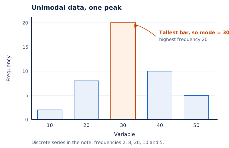
The horizontal axis is labelled Variable and the vertical axis Frequency. The outlined bars rise towards one tallest central bar and then fall, showing one prominent peak.
Drawn by One Young India. Reference: NCERT Class 11, unnumbered graph, p. 68
What the figure shows
Bimodal data
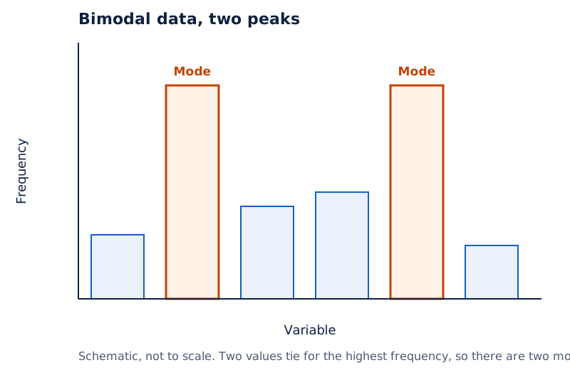
The axes again show Variable and Frequency. Two taller bars are separated by two lower bars, displaying two peaks rather than a single central peak.
Drawn by One Young India. Reference: NCERT Class 11, unnumbered graph, p. 68
These graphs illustrate why the number of concentrations matters. A single average may not express every feature of the distribution, particularly when values are concentrated around more than one point.
How is mode calculated for a continuous series?
The modal class is the class with the largest frequency. For a continuous series, the mode calculation requires equal class intervals and an exclusive series. If only midpoints are supplied, obtain the class intervals before calculating mode.
The formula is Mode = L + [D₁ / (D₁ + D₂)] × h. Here L now means the lower limit of the modal class, and h is the class width. D₁ and D₂ are frequency differences.
D₁ is the difference between the modal-class frequency and the preceding-class frequency, ignoring signs. D₂ is the difference between the modal-class frequency and the succeeding-class frequency, ignoring signs. Preceding and succeeding refer to the order of class values.
How do we convert cumulative frequencies?
A less-than cumulative frequency gives the number of observations below a stated upper limit. Subtract consecutive cumulative totals to obtain ordinary class frequencies. The greatest cumulative total is not the frequency of the modal class.
| Monthly income, thousand Rs | Less-than cumulative frequency | Corresponding income group, thousand Rs | Ordinary frequency |
|---|---|---|---|
| Less than 50 | 97 | 45 to 50 | 2 |
| Less than 45 | 95 | 40 to 45 | 5 |
| Less than 40 | 90 | 35 to 40 | 10 |
| Less than 35 | 80 | 30 to 35 | 20 |
| Less than 30 | 60 | 25 to 30 | 30 |
| Less than 25 | 30 | 20 to 25 | 18 |
| Less than 20 | 12 | 15 to 20 | 8 |
| Less than 15 | 4 | 10 to 15 | 4 |
The frequency for 25 to 30 is 60 − 30 = 30. This is the largest ordinary frequency, so 25 to 30 is the modal class. Its preceding class, 20 to 25, has frequency 18; its succeeding class, 30 to 35, has frequency 20.
Therefore L = 25, D₁ = 12, D₂ = 10 and h = 5. The expression to evaluate is 25 + [12 / (12 + 10)] × 5. Its unit is thousand Rs, which must remain the same throughout the calculation.
How should we choose and compare the three averages?
The appropriate average depends on the purpose of analysis and the nature of the distribution. A question about total values spread across observations differs from a question about the middle position or the most frequent category.
What are the merits and limitations of each measure?
| Measure | Useful feature | Feature to consider when choosing |
|---|---|---|
| Arithmetic mean | Simple to calculate and based on all observations | Unduly affected by extreme items |
| Median | Provides a better summary when extreme items affect the mean | Concentrates on the central items rather than all values |
| Mode | Generally used to describe qualitative data | May be non-unique or absent |
Qualitative data describes characteristics or categories, such as preferred shirt styles. Mode is generally used to describe such data. Keep “generally” in mind: choosing an average still requires attention to what information the comparison is intended to provide.
Median and mode can be computed graphically. They can also be computed in an open-ended distribution, in which an end class lacks one stated boundary. These features help distinguish them from an average based on adding all observed values.
How do their positions compare in the height illustration?
The heights shown are 54, 77, 67, 67, 46, 64, 62, 56 and 38 inches. Their mean is 59 inches. In ascending order, the middle height is 62 inches, while the repeated height 67 inches is the mode.
Using < to mean “less than”, this gives mean < median < mode. With > meaning “greater than”, the orders mean > median > mode and mean < median < mode place the median between the other two.
The three answers describe different aspects of the same observations. The mean uses their total, the median their ordered position, and the mode their repetition. The reason for summarising the data should guide which of these aspects receives emphasis.
Glossary
- Central tendency — A numerical summary that represents a collection of observations through a typical value.
- Arithmetic mean — The sum of all observed values divided by the total number of observations.
- Assumed mean — A chosen starting value used to simplify the calculation of arithmetic mean.
- Deviation — The signed difference between an observation and a specified reference value.
- Frequency — The number of times a value occurs in the observed data.
- Class midpoint — The value halfway between the lower and upper limits of a class.
- Weighted mean — An average calculated after assigning weights to values according to their importance.
- Median — The central positional value separating an ordered distribution into two equal parts.
- Cumulative frequency — The running total of frequencies up to a given value or class.
- Quartiles — Three dividing values that separate ordered observations into four equal parts.
- Percentiles — Dividing values that separate an ordered distribution into one hundred equal parts.
- Mode — The observed value that occurs most frequently in a distribution of data.
- Modal class — The class interval with the largest frequency in a continuous frequency distribution.
Common errors and misconceptions
- Misconception: Every average describes the same feature. Correct: Mean uses all values, median identifies the centre of ordered data, and mode identifies the most frequent value.
- Misconception: An assumed mean must occur in the data. Correct: Any value can be chosen, although a centrally located value can simplify the arithmetic.
- Misconception: A discrete mean is divided by the number of distinct values. Correct: Divide the sum of frequency-value products by total frequency.
- Misconception: The median position is the median value. Correct: Use the calculated position to locate the relevant observation or observations in the ordered series.
- Misconception: The median-class cumulative frequency enters the subtraction. Correct: Use the cumulative frequency of the class preceding the median class.
- Misconception: The greatest frequency is the mode. Correct: In a discrete series, the mode is the variable value corresponding to that frequency.
- Misconception: Mode must be unique. Correct: Data may have one mode, two modes, more than two modes, or no mode.
- Misconception: Deviations from any average sum to zero. Correct: The zero algebraic sum is a property of deviations from the arithmetic mean.
Exam-style questions with model answers
Q1. Define central tendency and name the three most commonly used measures. [2 marks]
- A measure of central tendency summarises a set of observations through one typical or representative value.
- The three most commonly used measures are arithmetic mean, median and mode, which describe different aspects of the data.
Q2. Calculate the arithmetic mean of economics test marks 40, 50, 55, 78 and 58, and interpret the result. [3 marks]
- The direct method adds all observations and divides by their number. Here there are five students, so the divisor is five.
- The total is 40 + 50 + 55 + 78 + 58 = 281. Dividing 281 by 5 gives a mean of 56.2 marks.
- The five students obtained 56.2 marks on average. This summarises the group, although no individual mark in the supplied list is 56.2.
Q3. A housing colony has 200 plots of 100 square metres, 50 plots of 200 square metres and 10 plots of 300 square metres. Calculate and interpret the mean plot size. [3 marks]
- Multiply each size by its frequency: 100 × 200 = 20000, 200 × 50 = 10000 and 300 × 10 = 3000 square metres.
- The total area is 33000 square metres and total number of plots is 260. Mean plot size = 33000 / 260 = 126.92 square metres.
- The average uses the number of plots in each size category. Dividing by the three categories would ignore the different frequencies and would not give the mean size per plot.
Q4. Find the median of the marks 25, 72, 28, 65, 29, 60, 30, 54, 32, 53, 33, 52, 35, 51, 42, 48, 45, 47, 46 and 33. Explain the method. [4 marks]
- Arrange the marks in ascending order: 25, 28, 29, 30, 32, 33, 33, 35, 42, 45, 46, 47, 48, 51, 52, 53, 54, 60, 65, 72.
- There are 20 observations, an even number. The median is therefore the arithmetic mean of the two middle observations.
- The tenth observation is 45 and the eleventh is 46. These are the values immediately on either side of the central position.
- Median = (45 + 46) / 2 = 45.5 marks. The answer is a mark, rather than the numerical position used to locate the middle.
Q5. Daily-wage classes, in Rs, are 20 to 25, 25 to 30, 30 to 35, 35 to 40, 40 to 45, 45 to 50, 50 to 55 and 55 to 60. Their worker frequencies are respectively 14, 28, 33, 30, 20, 15, 13 and 7. Find and interpret the median daily wage. [5 marks]
- Add the worker frequencies to obtain the total number of observations, N = 160. For this continuous series the required central position is N / 2 = 80.
- The ascending cumulative frequencies are 14, 42, 75, 105, 125, 140, 153 and 160. The 80th observation falls in the class 35 to 40.
- The median-class lower limit is 35, its frequency is 30, its width is 5, and the cumulative frequency of the preceding class is 75.
- Substitution gives median = 35 + [(80 − 75) / 30] × 5 = Rs 35.83. Use 75 in the subtraction, not the cumulative total including the median class.
- The median divides the distribution so that 50% of workers receive less than or equal to Rs 35.83 and 50% receive more than or equal to this daily wage.
Q6. Ten families have weekly incomes, in Rs, of 850, 700, 100, 750, 5000, 80, 420, 2500, 400 and 360. Calculate their arithmetic mean using an assumed mean of Rs 850. [5 marks]
- Use the assumed mean method: subtract the chosen starting value, Rs 850, from each income. Each difference is a deviation, retaining its positive or negative sign.
- The ten deviations, in the same order as the incomes, are 0, −150, −750, −100, +4150, −770, −430, +1650, −450 and −490.
- Add the signed deviations to obtain +2660. There are ten families, so the average deviation is 2660 / 10 = Rs 266.
- Add this correction to the assumed mean: arithmetic mean = 850 + 266 = Rs 1,116. The positive correction places the mean above the starting value.
- The families earn Rs 1,116 per week on average. This summarises all ten incomes and does not imply that each family earns exactly that amount.
Q7. Find the lower quartile of the marks 22, 26, 14, 30, 18, 11, 35, 41, 12 and 32. [3 marks]
- Arrange the ten marks in ascending order: 11, 12, 14, 18, 22, 26, 30, 32, 35, 41. This ordering is necessary because quartiles are positional values.
- The lower-quartile position is (10 + 1) / 4 = 2.75. It lies between the second item, 12, and third item, 14.
- Add three-quarters of their difference to the second value: lower quartile = 12 + 0.75 × (14 − 12) = 13.5 marks.
Q8. Explain three considerations in choosing between arithmetic mean, median and mode. [3 marks]
- Arithmetic mean is simple to calculate and uses all observations, but extreme items can unduly affect it. Consider whether such items make it a poor summary.
- Median is a better summary for data affected by extreme items because it concentrates on the central position rather than responding to every value.
- Mode is useful for the most frequently occurring value and is generally used for qualitative data. The purpose of analysis and nature of the distribution guide the choice.
Key takeaways
- Central tendency condenses observations into a representative value, but the choice of average depends on the question being investigated.
- Arithmetic mean uses all observations, while assumed mean and step deviation simplify its calculation without changing the measure.
- Frequency must be included in grouped calculations, and class midpoints represent continuous intervals when calculating their arithmetic mean.
- Deviations from arithmetic mean sum to zero, but extreme observations can unduly affect the mean.
- Median requires ordered data; an even number of individual observations requires averaging the two middle values.
- Quartiles divide ordered observations into four parts, while percentiles divide the distribution into one hundred equal parts.
- Mode identifies the most frequent value, and a distribution can have multiple modes or no mode.
- Continuous mode calculations require equal exclusive class intervals and the frequencies of the modal class and its neighbours.
Test yourself
What does ΣX mean in the direct-method formula?
It means the sum of all observed values; Σ is the symbol for summation.
Must an assumed mean be one of the observations?
No. Any value can be chosen, although a centrally located value can make calculation easier.
Why is the common factor multiplied back in step deviation?
It restores the scale of the deviations before their average is added to the assumed mean.
Which position locates the median class in a continuous series?
Use N / 2, where N is total frequency, and locate that observation through cumulative frequency.
Which cumulative frequency enters the grouped median formula?
Use the cumulative frequency of the class preceding the median class, not the total including it.
What do Q₂ and P₅₀ have in common?
Both identify the median, the central dividing value of the ordered distribution.
For values 10, 20, 30, 40, 50 with frequencies 2, 8, 20, 10, 5, what is the mode?
The mode is 30, the variable value corresponding to the largest frequency of 20.
Why does the series 1, 1, 2, 2, 3, 3, 4, 4 have no mode?
Every distinct value occurs equally often, so no value occurs more frequently than the others.
Write about it
Turn a question from this chapter into a paper.
The Writing Studio has a structure guide, a rubric and citation tools for 15 formats, from essays to research papers. Drafting is free with an account. Learnacy Essential adds feedback from an AI writing coach and submission to The OYI Review.
Learnacy Essential is ₹1,499 for the year. Publication depends on review and is not guaranteed.