
Organisation of Data | CBSE Class 11 Economics Notes
On this page
This note covers raw data, the purpose and types of classification, continuous and discrete variables, frequency distributions, class limits, class marks, inclusive and exclusive intervals, tally marking, unequal classes, loss of information, frequency arrays and bivariate distributions.
Why do raw data need organisation?
Definition: Classification means arranging or organising things into groups or classes on the basis of some criteria. Raw data are data that have not yet been classified.
Raw data are often very large and cumbersome to handle. Finding useful information in a disorganised collection can be tedious. Organisation brings order to the data and prepares them for further statistical analysis.
How does classification help in everyday life?
A kabadiwallah, or junk dealer, groups newspapers, plastics, glass and metals separately. Within metals, articles may be sorted into iron, copper, aluminium and brass. This arrangement makes it easier to find an item that a buyer wants.
The basis of grouping serves a purpose. The dealer groups goods according to the markets for reused materials. Empty bottles, broken mirrors and windowpanes belong together under glass. Classification therefore involves a relevant criterion, rather than an arbitrary arrangement.
Schoolbooks can similarly be arranged by subject. A history book can then be found among the history books instead of searching the entire collection. The same books could also be arranged alphabetically by author or according to their year of publication.
What changes when data are classified?
Consider marks in mathematics collected for 100 students, or monthly food expenditure collected for 50 households. An unordered list preserves the individual records, but it does not make the overall pattern easy to understand.
Classification places facts with similar characteristics together. It summarises the collection, helps comparison and makes it easier to draw inferences. The method chosen depends on the purpose of the enquiry, such as understanding how students have performed in mathematics.
A larger collection makes organisation still more useful. Handling marks for 1,000 students would be more tedious than handling marks for 100. Likewise, locating information about expenditure becomes harder when the number of households increases from 50 to 5,000.
How do chronological and spatial classifications differ?
Chronological classification arranges data with reference to time. The order may be ascending, from earlier to later periods, or descending, from later to earlier periods. Years, quarters, months and weeks can provide the time units.
A time series is a series of values for different times. Population recorded for successive years is an example. The following figures illustrate India's population arranged chronologically. Population is expressed in crores; one crore means ten million.
| Year | Population of India, in crores |
|---|---|
| 1951 | 35.7 |
| 1961 | 43.8 |
| 1971 | 54.6 |
| 1981 | 68.4 |
| 1991 | 81.8 |
| 2001 | 102.7 |
| 2011 | 121.0 |
What makes a classification spatial?
Spatial classification arranges data with reference to geographical locations, such as countries, states, cities or districts. The distinguishing feature is the location attached to each value, rather than a sequence of dates.
The wheat figures below are spatially classified because they refer to different countries in 2013. Yield here means wheat output per unit of land area. The unit kg/hectare means kilograms per hectare.
| Country | Wheat yield in 2013, kg/hectare |
|---|---|
| Canada | 3594 |
| China | 5055 |
| France | 7254 |
| Germany | 7998 |
| India | 3154 |
| Pakistan | 2787 |
The organising question therefore differs between these two arrangements. A chronological table asks how the recorded value differs across time periods. A spatial table identifies values belonging to different places. Both bring order to data, but they use different criteria.
The presence of numbers does not by itself identify the classification. Both tables contain numerical values. The first arranges its entries by year, while the second associates the entries with countries during the same stated year.
What distinguishes qualitative from quantitative classification?
Qualities or attributes are characteristics that cannot be expressed quantitatively. Examples include nationality, literacy, religion, gender and marital status. These attributes are classified by their presence or absence, rather than measured as numerical magnitudes.
Definition: Qualitative classification groups data according to attributes. Quantitative classification groups data according to characteristics that can be expressed numerically, such as height, weight, age, income and marks.
How can an attribute be subdivided?
A qualitative classification can proceed in stages. In the population example, the first division is into male and female categories. Each category is then subdivided into married and unmarried groups, using marital status as the second attribute.
The second division does not replace the first. It gives further groups within each of the initial categories. Thus the criterion used at one stage can differ from the criterion used at the next stage of classification.
How does a numerical characteristic form classes?
Quantitative classification uses numerical characteristics such as marks obtained by students. Marks can be grouped into classes, and the number of students in each class can then be recorded. This summarises how the marks are distributed.
The essential distinction concerns the characteristic used for grouping. Literacy and marital status are attributes; height and income are quantitative characteristics. A count of people in a qualitative category does not turn the original attribute into a numerical measurement.
The choice of classification follows the purpose of the study. Population can be organised by attributes such as education, marital status and occupation. Such grouping helps reveal the structure of a large collection of population records.
How do continuous and discrete variables differ?
A variable is a characteristic whose value can vary. An observation is a recorded value of the characteristic. Variables are broadly classified as continuous or discrete according to the values they can take.
What is a continuous variable?
A continuous variable can take any numerical value within its range of variation. Its values can include whole numbers, fractions and values that are not exact fractions. It can vary through intermediate values rather than move only between separate permitted values.
Height illustrates continuity. As a student's height changes from 90 to 150 centimetres, it can pass through the values between them. Possible heights include 90.85, 102.34 and 149.99 centimetres. Weight, time and distance are other continuous variables.
Can a discrete variable have fractional values?
A discrete variable takes only certain values and changes by finite jumps. It does not take intermediate values between adjacent permitted values. The number of students in a class, for example, may be 25 or 26 but cannot be 25.5.
However, discreteness does not mean that fractions are forbidden in every case. Let X denote a variable restricted to the values 1/8, 1/16, 1/32, 1/64 and so on. X is discrete because it cannot take values between adjacent permitted fractions.
Note: Decide whether a variable is discrete by examining its possible values and the gaps between them. Do not classify it merely by checking whether a fraction appears.
Marks recorded only as full numbers provide a discrete example when fractional marks are not allowed. Height and weight provide continuous examples. The rules governing the possible observations matter when choosing how to group the data.
What does a frequency distribution show?
Frequency means the number of times an observation occurs. A frequency distribution organises the values of a quantitative variable into classes and shows the number of observations belonging to each class.
Class frequency is the number of values in a particular class. It differs from the frequency of one exact value. A class can contain several different observed values, while its frequency counts all the observations assigned to it.
The marks distribution below groups the marks of 100 students. It also shows each class mark, the midpoint used to represent a class. The method for calculating this midpoint is explained in the next section.
| Marks class | Frequency | Class mark |
|---|---|---|
| 0 to 10 | 1 | 5 |
| 10 to 20 | 8 | 15 |
| 20 to 30 | 6 | 25 |
| 30 to 40 | 7 | 35 |
| 40 to 50 | 21 | 45 |
| 50 to 60 | 23 | 55 |
| 60 to 70 | 19 | 65 |
| 70 to 80 | 6 | 75 |
| 80 to 90 | 5 | 85 |
| 90 to 100 | 4 | 95 |
The total frequency, obtained by adding the class frequencies, is 100. The class 50 to 60 has the maximum concentration, with 23 observations. The class 0 to 10 has the minimum concentration, with one observation.
Note: In this marks distribution, a score of 40 belongs to 40 to 50. The final class 90 to 100 includes the observed score 100.
What is relative frequency?
Relative frequency expresses frequency as a proportion or percentage of total frequency. It relates the number in one class to the whole collection, making the concentration of observations in that class explicit.
For these 100 students, the classes 40 to 50, 50 to 60 and 60 to 70 contain 21, 23 and 19 observations respectively. Together, these classes contain 63 students, or 63 per cent of all observations.
How are class limits, widths and class marks calculated?
Class limits are the two ends of a class. The lower end is its lower class limit, and the upper end is its upper class limit. For the class 60 to 70, these limits are 60 and 70.
What is class width?
Class interval, also called class width, is the difference between the upper and lower class limits. It describes the size of the interval rather than the number of observations within it.
Class width = Upper class limit − Lower class limit
Worked example 1. Find the class width for the marks class with lower limit 60 and upper limit 70.
Answer: Class width = 70 − 60 = 10 marks. The subtraction uses the two class limits; it does not use the class frequency.
How is the midpoint found?
Class mark = (Upper class limit + Lower class limit)/2
The slash in this formula denotes division. The class mark lies halfway between the two limits. It is also called the class midpoint or mid-value, and represents the observations after they have been grouped into the class.
Worked example 2. Find the class mark for the class 60 to 70.
Answer: Class mark = (70 + 60)/2 = 65 marks. This is the value representing the class in further calculations based on the grouped distribution.
Width and midpoint answer different questions. Width measures the distance between class limits; the midpoint locates the centre. In the same class, the width is 10 while the midpoint is 65. Neither number states how many observations belong to the class.
Once raw data are grouped, further calculations use class marks instead of individual observations. This convention is useful for summarising data, but it also explains why grouping involves a loss of information about the original values.
How should the number and size of classes be chosen?
Constructing a frequency distribution involves related decisions. The classes must organise the data usefully, and the class limits should be definite and clearly stated. The following questions guide the construction.
- Should the class intervals have equal or unequal sizes?
- How many classes should be formed?
- What should the size of each class be?
- How should the class limits be determined?
- How should the frequency of each class be obtained?
How does the range guide the choice?
Range is the difference between the largest and smallest values of the variable. It gives the span of values that the classification must cover.
Range = Largest value − Smallest value
The number of classes is usually between six and fifteen. With equal class intervals, dividing the range by the class width gives the number of classes. The choice of width and the choice of number of classes are therefore interlinked.
Number of classes = Range/Class width
Worked example 3. The marks range from 0 to 100. If ten equal classes are chosen, find the range and the width of each class.
Answer: Range = 100 − 0 = 100 marks. Class width = 100/10 = 10 marks. Ten equal intervals therefore cover the stated range.
When are unequal intervals useful?
Unequal class intervals are useful when the range is very high, as can happen with incomes. Moderate equal intervals would produce many classes. Large equal intervals would tend to suppress information about very small or very high incomes.
Unequal intervals are also useful when many values are concentrated in a small part of the range. Equal intervals would then lead to a lack of information about many values. In other cases, equal intervals are used.
Open-ended classes leave one end unspecified, as in “70 and over” or “less than 10”. Generally, such classes are not desirable. Class limits should encourage observations to concentrate around the middle of each interval.
How do inclusive and exclusive class intervals work?
Class limits alone do not settle where a boundary value belongs. The method of including or excluding endpoints must also be specified. This is particularly important when adjacent classes share a numerical endpoint.
What is the inclusive method?
Under the inclusive method, values equal to both the lower and upper limits belong to the same class. For marks recorded only in full numbers, classes can be written as 0 to 10, 11 to 20, 21 to 30 and so on.
In this arrangement, both 0 and 10 belong to the first class. The next class begins at 11. The form is being applied to marks for which fractional observations are not allowed.
What is the exclusive method?
Under the exclusive method, a value equal to either the upper or lower limit is excluded from that class. Classes may be written as 0 to 10, 10 to 20 and 20 to 30, but the endpoint convention must be decided beforehand.
With the upper limit excluded, 10 belongs to 10 to 20 and 30 belongs to 30 to 40. With the lower limit excluded, 10 belongs to 0 to 10 and 30 belongs to 20 to 30.
Note: Exclusive classification does not necessarily mean excluding the upper limit. Either endpoint can be excluded, provided the convention is decided in advance and used consistently.
Both inclusive and exclusive intervals can be used for discrete variables. For continuous variables, inclusive class intervals are used very often, with attention to continuity when the displayed limits leave gaps.
A continuous weight interval can be understood as 30 kilograms and above but under 40 kilograms. The next interval is 40 kilograms and above but under 50 kilograms. This wording makes clear which class receives the shared boundary value.
How are gaps between inclusive intervals adjusted?
Inclusive intervals can leave a gap between an upper limit and the next lower limit. Income is a continuous variable, so such gaps require attention. For example, the adjacent income classes 800 to 899 and 900 to 999 have a gap of 1 rupee.
What are the steps in adjustment?
- Subtract the upper limit of the first class from the lower limit of the second class: 900 − 899 = 1.
- Divide this difference by two: 1/2 = 0.5.
- Subtract 0.5 from the lower limit of every class.
- Add 0.5 to the upper limit of every class.
The resulting adjusted limits restore continuity. The upper limit of one class meets the lower limit of the next class. The frequencies remain those of the original income distribution of 550 employees.
| Original income class, rupees | Adjusted income class, rupees | Employees |
|---|---|---|
| 800 to 899 | 799.5 to 899.5 | 50 |
| 900 to 999 | 899.5 to 999.5 | 100 |
| 1000 to 1099 | 999.5 to 1099.5 | 200 |
| 1100 to 1199 | 1099.5 to 1199.5 | 150 |
| 1200 to 1299 | 1199.5 to 1299.5 | 40 |
| 1300 to 1399 | 1299.5 to 1399.5 | 10 |
| Total | All classes | 550 |
Worked example 4. Adjust the adjacent income classes Rs 800 to Rs 899 and Rs 900 to Rs 999 to remove their gap. Here Rs denotes rupees.
Answer: The gap is 900 − 899 = 1 rupee, and half the gap is 0.5 rupee. Subtracting 0.5 from each lower limit and adding 0.5 to each upper limit gives Rs 799.5 to Rs 899.5 and Rs 899.5 to Rs 999.5.
How is the adjusted midpoint obtained?
The adjusted class mark is the sum of the adjusted upper and lower class limits divided by two. The midpoint rule is unchanged in form; the calculation now uses the adjusted endpoints.
The adjustment concerns the boundaries of the classes. It does not add employees or remove them from the distribution. Keeping the original frequencies alongside both sets of limits makes that distinction clear.
How do tally marks help, and what information does grouping lose?
A tally mark is a stroke used to count an observation against its class. For each student, identify the appropriate marks class and place one tally against it. The class frequency equals the number of tallies in that class.
How are observations assigned?
A score of 57 receives a tally against 50 to 60. A score of 71 receives a tally against 70 to 80. With the upper limit excluded, a score of 40 receives a tally against 40 to 50.
Four tally strokes are drawn together, and the fifth crosses them. The tallies can then be counted in groups of five. For 16 observations, the arrangement consists of three groups of five and one additional stroke.
Distinguish an exact-value count from a class count. In the marks data, the value 40 occurs three times. The frequency of a broader class counts all its observations, including observations with different values inside that interval.
Why does grouping lose information?
Loss of information means that the grouped distribution no longer displays the actual values of the individual observations. It retains the number in each class and uses the class mark to represent them in subsequent calculations.
The class 20 to 30 contains six observations: 25, 25, 20, 22, 25 and 28. Its frequency is 6, and its class mark is 25. The grouped entry therefore replaces the separate values with a class and its frequency.
For further calculations using this grouped distribution, all values in the class are assumed equal to 25. This does not mean that every student actually scored 25. It is the representation adopted after grouping.
The advantage is that classification makes a large collection concise and comprehensible. The limitation is that the individual detail is lost. The gain in making sense of raw data compensates for this loss.
How do unequal classes change the frequency curve?
A frequency curve represents a frequency distribution graphically. Class marks are plotted on the X-axis, the horizontal axis, and frequencies on the Y-axis, the vertical axis. The curve shows how the frequencies vary across the class marks.
What the figure shows
Equal-class frequency curve
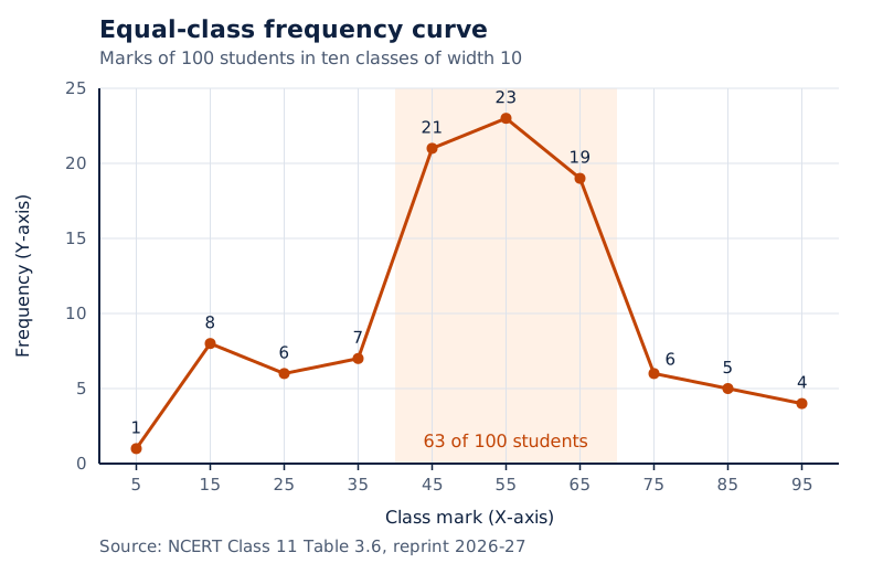
The plotted line rises in the middle of the horizontal scale, reaches its highest point near class mark 55, and falls towards the higher class marks. The grid shows frequencies vertically.
Drawn by One Young India. See Fig. 3.1 in your NCERT textbook
Why split the middle classes?
In the marks distribution, most observations are concentrated in 40 to 50, 50 to 60 and 60 to 70. Their frequencies are 21, 23 and 19. Thus 63 per cent lie in this middle range, while the remaining 37 per cent lie in the other classes.
Splitting each middle class into two gives intervals of width 5. The other classes retain width 10. The following table shows the smaller middle classes, their frequencies and their new class marks.
| Marks class | Frequency | Class mark |
|---|---|---|
| 40 to 45 | 9 | 42.5 |
| 45 to 50 | 12 | 47.5 |
| 50 to 55 | 7 | 52.5 |
| 55 to 60 | 16 | 57.5 |
| 60 to 65 | 10 | 62.5 |
| 65 to 70 | 9 | 67.5 |
The aim is to make class marks come as close as possible to the values around which observations in each class tend to concentrate. In these subdivided classes, the new marks are more representative than the old marks.
What the figure shows
Unequal-class frequency curve
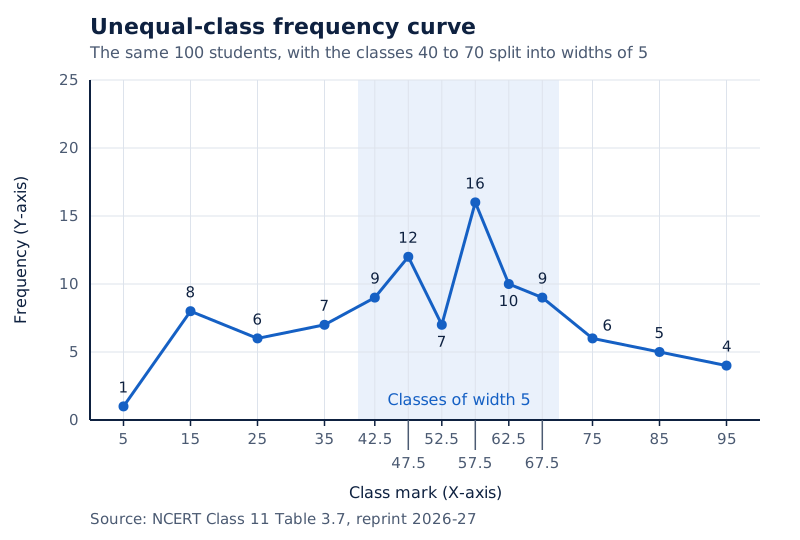
The horizontal scale carries the class marks and the vertical scale carries frequency. In the middle, the line rises, dips, rises to a sharper peak and then falls as it moves towards higher class marks.
Drawn by One Young India. See Fig. 3.2 in your NCERT textbook
The change in grouping changes the information displayed by the curve. Smaller middle intervals reveal differences that the broader classes combined. The observations remain the same; the classes and the representative midpoints have changed.
What are frequency arrays and bivariate distributions?
How does a frequency array organise discrete values?
A frequency array classifies the values of a discrete variable by showing the frequency corresponding to each value. Household size, meaning the number of people in a household, illustrates a variable with whole-number values.
| Household size | Number of households |
|---|---|
| 1 | 5 |
| 2 | 15 |
| 3 | 25 |
| 4 | 35 |
| 5 | 10 |
| 6 | 5 |
| 7 | 3 |
| 8 | 2 |
| Total | 100 |
Read a row by separating the value from its frequency. The row for household size 4 means that 35 households have four members each. Here, 4 is a value of the variable, while 35 is its frequency.
How does a bivariate distribution differ from a univariate distribution?
A univariate frequency distribution concerns one variable. A bivariate frequency distribution concerns two variables together.
A sample is a set of units selected from a population, the whole collection under study. Very often, more than one type of information is collected for each sampled unit. For example, sales and advertisement expenditure can be recorded for 20 companies in a city.
In a bivariate table, classes of sales appear in columns and classes of advertisement expenditure in rows. A cell, the position where a row and column meet, gives the number of firms belonging to both corresponding classes.
A lakh means one hundred thousand. In the company example, one cell contains 3 firms with sales between Rs 135 lakh and Rs 145 lakh and advertisement expenditure between Rs 64 thousand and Rs 66 thousand. Sales and advertisement expenditure use different monetary scales.
The cell frequency is a joint count. It describes firms satisfying both the sales classification and the expenditure classification. By contrast, a univariate distribution summarises how the observations are distributed with respect to one variable at a time.
Glossary
- Raw data — Unclassified observations that require organisation before their overall pattern can be understood easily.
- Classification — Arranging things or observations into groups according to a chosen criterion.
- Chronological classification — Organisation of data with reference to time, in ascending or descending order.
- Spatial classification — Organisation of data with reference to geographical locations such as countries or states.
- Attribute — A qualitative characteristic, such as literacy or marital status, that is not measured numerically.
- Continuous variable — A variable capable of taking intermediate numerical values throughout its range of variation.
- Discrete variable — A variable taking separate permitted values without taking values between adjacent possibilities.
- Class frequency — The number of observations assigned to a particular class in a frequency distribution.
- Class limits — The lower and upper endpoints that specify a class in a distribution.
- Class width — The difference obtained by subtracting the lower class limit from the upper class limit.
- Class mark — The midpoint of a class, used to represent its observations in grouped calculations.
- Range — The difference between the largest and smallest values of a variable.
- Relative frequency — Frequency expressed as a proportion or percentage of the total frequency.
- Frequency array — An arrangement showing the frequencies corresponding to the individual values of a discrete variable.
- Bivariate distribution — A frequency distribution that classifies observations with reference to two variables together.
Common errors and misconceptions
- Misconception: A discrete variable cannot take fractional values. Correct: It can take specified fractions, provided it cannot take intermediate values between adjacent permitted values.
- Misconception: Every exclusive distribution excludes the upper limit. Correct: Either the upper or lower limit may be excluded; the convention must be decided beforehand.
- Misconception: Class frequency and class width mean the same thing. Correct: Frequency counts observations; width is the difference between the class limits.
- Misconception: A class mark records every actual observation in that class. Correct: It is a midpoint used to represent the grouped observations in further calculations.
- Misconception: All frequency distributions must use equal intervals. Correct: Unequal intervals are useful for very wide ranges or concentrations within a small part of the range.
- Misconception: Adjusting inclusive limits changes the employee frequencies. Correct: The adjustment restores continuity between the income intervals while retaining their frequencies.
- Misconception: A bivariate cell counts observations for either one of its two classes. Correct: It counts observations belonging to the corresponding row and column classes together.
Exam-style questions with model answers
Q1. Define classification and give one advantage of classifying raw data. [2 marks]
- Classification means arranging observations into groups or classes according to a chosen criterion.
- It makes raw data more comprehensible, allowing similar observations to be located and compared more easily.
Q2. Height can take all intermediate values as it changes, while a variable X is restricted to 1/8, 1/16, 1/32, 1/64 and so on. Distinguish continuous and discrete variables, and explain why X is discrete despite its fractional values. [3 marks]
- A continuous variable can take intermediate numerical values within its range. Height, for example, can vary through whole-number and fractional values.
- A discrete variable takes only certain values and changes in jumps, without taking values between adjacent permitted values.
- A variable restricted to 1/8, 1/16, 1/32, 1/64 and so on is discrete. Although these are fractions, the variable cannot take intermediate values between adjacent permitted fractions.
Q3. A marks distribution has smallest value 0, largest value 100 and ten equal classes. For its class 60 to 70, calculate the range, class width, class mark and state the use of the class mark. [4 marks]
- The range is the largest value minus the smallest value: 100 − 0 = 100 marks.
- The class width is 100 divided by ten classes, giving 10 marks. For 60 to 70, it is also 70 − 60 = 10.
- The class mark is the average of the two limits: (70 + 60)/2 = 65 marks.
- The class mark represents the observations in the class when further calculations are made using the grouped distribution.
Q4. Inclusive income classes are Rs 800 to Rs 899 and Rs 900 to Rs 999, containing 50 and 100 employees respectively. Show how to adjust the limits for continuity and state what happens to the frequencies. [5 marks]
- The gap is the next lower limit minus the preceding upper limit. For the given classes, it is 900 − 899 = 1 rupee.
- Half the gap is 1/2 = 0.5 rupee. This amount is used to adjust both ends of each interval.
- Subtracting 0.5 from the lower limits gives Rs 799.5 and Rs 899.5 as the new lower limits.
- Adding 0.5 to the upper limits gives Rs 899.5 and Rs 999.5. The adjusted classes therefore meet at Rs 899.5.
- The frequencies remain 50 and 100 employees respectively. The boundary adjustment restores continuity; it does not alter the number of employees represented in each class.
Q5. The marks 25, 25, 20, 22, 25 and 28 are grouped in the class 20 to 30. Explain the loss of information, giving the frequency, class mark, treatment in further calculations and the benefit of grouping. [5 marks]
- There are six observations in the stated list, so the class frequency is 6. This counts all the records belonging to the interval.
- The class mark is the average of the limits: (30 + 20)/2 = 25. It is the representative midpoint of the class.
- The grouped entry records the class and its frequency rather than the separate marks 25, 25, 20, 22, 25 and 28.
- Further calculations using the grouped distribution treat these values as equal to the class mark, 25. Their individual differences are therefore lost.
- The benefit is a concise and comprehensible summary. Grouping makes the data easier to handle, although it sacrifices the detailed values contained in the original list.
Q6. The adjacent classes are 0 to 10 and 10 to 20. Explain where a value of 10 belongs under each exclusive convention, and define the inclusive method. [3 marks]
- If the upper limit is excluded, 10 does not belong to 0 to 10. It belongs to the next class, 10 to 20.
- If the lower limit is excluded, 10 belongs to 0 to 10 and is excluded from the class beginning at 10.
- Under the inclusive method, both lower and upper limits belong to their own class. The endpoint convention therefore needs to be clear when classes are constructed.
Q7. In a distribution of 100 students, the classes 40 to 50, 50 to 60 and 60 to 70 have frequencies 21, 23 and 19. Explain their combined concentration and why they might be subdivided into classes of width 5. [3 marks]
- The three classes contain 21 + 23 + 19 = 63 students out of the total of 100 students.
- Thus 63 per cent of the observations are concentrated in this middle range. This is most of the given observations.
- Subdividing these classes into intervals of width 5 gives more detail within the concentration. The new class marks can lie closer to the values around which observations tend to concentrate.
Q8. In a bivariate table, sales classes form columns and advertisement expenditure classes form rows. A cell for sales of Rs 135 to Rs 145 lakh and expenditure of Rs 64 to Rs 66 thousand contains 3. Interpret it. [2 marks]
- The cell represents 3 firms whose sales fall between Rs 135 lakh and Rs 145 lakh.
- Those same firms have advertisement expenditure between Rs 64 thousand and Rs 66 thousand, so both conditions hold together.
Key takeaways
- Classification brings order to raw data by grouping observations according to a criterion suited to the enquiry.
- Chronological classification uses time, spatial classification uses place, and qualitative classification uses attributes rather than numerical measurements.
- Continuous variables admit intermediate values; discrete variables move between separate permitted values, which can sometimes be fractions.
- Class width is the difference between the limits, while the class mark is their average.
- Inclusive intervals include both endpoints; exclusive intervals exclude either the upper or lower endpoint according to a stated convention.
- Adjust inclusive intervals by half the gap between adjacent limits to restore continuity while retaining class frequencies.
- Grouping makes data concise but loses individual detail because further grouped calculations use class marks.
- A frequency array records discrete values and their frequencies; a bivariate distribution classifies two variables together.
Test yourself
What determines the criterion used to classify a collection?
The purpose of the enquiry determines the criterion, such as subject for books or time for a time series.
Why is the number of students in a class discrete?
It takes whole-number counts, such as 25 or 26, without taking intermediate values such as 25.5.
What is the class mark of the interval 40 to 50?
The class mark is (50 + 40)/2 = 45, the midpoint used to represent the class.
What does a tally mark record?
It records one observation assigned to a class; counting that class's tallies gives its frequency.
Why should “usually six to fifteen classes” not be treated as a fixed requirement?
The word “usually” expresses a general guideline. Class number and width are linked to the range and the chosen grouping.
Which axes carry class marks and frequencies in a frequency curve?
Class marks are plotted on the horizontal X-axis and frequencies on the vertical Y-axis.
What is lost when observations are replaced by a class mark?
The separate observed values are no longer used in further grouped calculations, so individual detail is lost.
How many variables does a bivariate frequency distribution organise?
It organises two variables together, showing the frequency for each corresponding pair of row and column classes.
Write about it
Turn a question from this chapter into a paper.
The Writing Studio has a structure guide, a rubric and citation tools for 15 formats, from essays to research papers. Drafting is free with an account. Learnacy Essential adds feedback from an AI writing coach and submission to The OYI Review.
Learnacy Essential is ₹1,499 for the year. Publication depends on review and is not guaranteed.