
Supply | ISC Class 12 Economics Notes
On this page
Watch & explore
Start with a few high-quality watches, then dive into the notes below.
Try an idea before you read. Step into the role of an agricultural producer to evaluate decisions regarding stock, supply, and crop allocation. Explore →
Learnacy Labs Try it hands-on: open the Markets lab
This note covers the meaning of supply, stock and supply, supply functions and schedules, the law of supply, determinants, movements and shifts of supply curves, exceptions, market supply, degrees of elasticity, and the percentage and geometric methods of measuring elasticity of supply.
What is supply, and how does it differ from stock?
Definition: Supply refers to the quantity of a commodity that a seller is willing and able to offer for sale at a given price during a specified period.
A commodity is a good offered in a market. The quantity supplied must be connected with both a price and a period. A statement about goods available with a seller does not, by itself, tell us how much the seller will offer for sale.
What does stock mean?
Stock is the total quantity of a commodity available with a seller at a particular time. Supply is the part offered for sale at the stated price during the relevant period. Availability and willingness to sell are therefore different ideas.
The distinction is between the quantity potentially available and the quantity actually offered. “Actual supply” does not mean that every unit offered has already found a buyer. Completed sales also depend on the buyers' willingness to purchase.
| Basis | Stock | Supply |
|---|---|---|
| Meaning | Quantity available with the seller | Quantity offered for sale at a stated price |
| Time reference | Measured at a particular time | Stated for a specified period |
| Decision involved | Goods are available | The seller is willing and able to sell them |
The cricket-ball example used below illustrates supply: firms offer 200 cricket balls when the price is 10 rupees per ball. The abbreviation Rs denotes rupees. That information identifies the quantity supplied at that price; it does not establish the total stock of cricket balls held by those firms.
Supply and quantity supplied also require care. A quantity supplied is one amount corresponding to one price. A supply schedule or curve describes the relationship across different prices, with the other determinants held constant.
How do a supply function, schedule and curve describe supply?
A supply function expresses how quantity supplied depends on its determinants. A unit tax is a tax per unit sale of output. A determinant is a factor that influences the seller's supply decision. These include the commodity's own price and the prices of inputs, meaning resources used in production. Technology means the methods of producing output. Taxes and the number of firms also affect market supply.
Write Qₛ = f(P, C, T, U, N), where Qₛ is quantity supplied, P is the commodity's price, C represents input prices, T represents technology, U represents a unit tax, and N is the number of firms. The symbol f means “is a function of”.
This notation organises the determinants; it does not specify their numerical effects. For an individual firm, N is omitted. To examine the relationship between the commodity's price and quantity supplied, hold the other determinants unchanged.
How is a schedule read?
A supply schedule lists prices and the quantities supplied at those prices. The following schedule describes one firm. Rs means rupees, and each quantity is measured in units of the same good over the same period.
| Price (Rs per unit) | Quantity supplied (units) |
|---|---|
| 0 | 0 |
| 1 | 0 |
| 2 | 0 |
| 3 | 1 |
| 4 | 2 |
| 5 | 3 |
| 6 | 4 |
A supply curve represents the same relationship graphically. Quantity goes on the horizontal axis and price on the vertical axis. Each price-quantity pair becomes a point. The zero entries show that positive production need not occur at every positive price.
Diagram
A supply schedule plotted
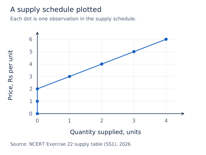
Label the horizontal axis “Quantity supplied, units” and the vertical axis “Price, Rs per unit”. Plot the pairs in the table, keeping quantity as the horizontal coordinate. The positive-output observations rise from left to right.
Drawn by One Young India.
The schedule and curve are alternative presentations of one relationship. Reading a point gives quantity at a particular price; comparing points shows how that quantity responds when price changes.
What does the law of supply state, and why does it operate?
Definition: The law of supply states that, other things remaining the same, quantity supplied rises when the commodity's price rises and falls when its price falls.
The condition ceteris paribus means “other things remaining the same”. In applying the law, hold constant the conditions that determine the supply curve. A simultaneous change in production costs cannot simply be treated as the effect of a change in the commodity's own price.
How do costs help explain the relationship?
Marginal cost, abbreviated MC, is the addition to total cost from producing one extra unit. A firm seeking the greatest profit, the excess of sales revenue over production costs, compares the extra revenue from selling output with the extra cost of producing it. Revenue means receipts from sales.
In perfect competition, an individual firm is a price-taker: it accepts the market price. For a price-taking firm, the extra revenue from another unit equals that price. Along the relevant rising marginal-cost curve, a higher price supports a larger profit-maximising output.
For positive production, the relationship P = MC identifies the equality of price and marginal cost. This equality alone is not sufficient: marginal cost must be non-decreasing at the chosen output, and price must cover the relevant average cost. Average cost means cost per unit of output.
In the short run, a period in which some production inputs are fixed, the firm produces zero output if price is below its minimum average variable cost. Average variable cost is variable cost per unit of output; variable costs change with production.
Therefore, an upward supply relationship does not mean every small price rise must produce additional output at every starting point. Both prices may remain below the threshold for production. The positive-output portion of the competitive firm's supply curve follows the relevant rising marginal-cost segment.
The law describes a conditional price response. It does not claim that price explains every observed change in output, or that all goods and all time periods allow the same adjustment.
Which factors change a firm's supply?
The determinants of supply explain why a firm may supply different quantities even when the commodity's market price remains unchanged. Because the competitive firm's supply curve is related to marginal cost, changes affecting marginal cost can change its supply curve.
How does technological progress affect supply?
Technological progress can allow the same capital and labour to produce more output. Capital refers here to produced means of production, while labour is human productive effort. An organisational innovation can also allow a given output to be made with fewer inputs.
It is expected that this will lower marginal cost at any level of output. The marginal-cost curve shifts rightward or downward, and the supply curve shifts rightward. At a given market price, the firm now supplies more output.
How do input prices affect supply?
Inputs are resources used in production. If an input price, such as the wage rate paid for labour, increases, production becomes more costly. The increase in average cost is usually accompanied by an increase in marginal cost at any level of output.
The marginal-cost curve then shifts leftward or upward, and supply shifts leftward. At the same market price, the firm supplies fewer units. A decrease in input prices is expected to shift supply rightward.
| Change | Cost effect | Supply effect |
|---|---|---|
| Technological progress | Marginal cost is expected to fall | Rightward shift |
| Increase in input prices | Marginal cost usually rises with average cost | Leftward shift |
| Imposition of a unit tax | Cost increases per unit | Leftward shift |
A unit tax is a tax imposed per unit sale of output. Unlike a movement caused by the selling price itself, this changes the cost conditions behind the supply decision. Its effect can be traced while holding the selling price constant.
The distinction between a cause and its consequence matters: a higher wage is an input-price change, whereas a higher price received for the finished good is a movement along the existing supply curve.
How do movements along a supply curve differ from shifts?
A movement along the supply curve occurs when the commodity's own price changes and the other determinants remain unchanged. An upward movement is an extension of supply; a downward movement is a contraction of supply. The existing curve contains both positions.
A shift of the supply curve occurs when a non-price determinant changes. “Non-price” here means something other than the commodity's own selling price. Input prices still qualify as determinants capable of shifting the curve.
A rightward shift is an increase in supply: more is supplied at a given price. A leftward shift is a decrease in supply: less is supplied at that same price. Compare quantities at a common price to identify the direction.
| Situation | Cause | Graphical change |
|---|---|---|
| Extension | Own price rises | Upward movement on one curve |
| Contraction | Own price falls | Downward movement on one curve |
| Increase in supply | For example, technological progress | Rightward shift of the curve |
| Decrease in supply | For example, a unit tax is imposed | Leftward shift of the curve |
How does a tax illustrate a shift?
Worked example 1. A unit tax of Rs 2 is imposed on a good. A firm produces and sells 10 units. Calculate its total tax payment.
Answer: Total tax = tax per unit × units sold = Rs 2 × 10 = Rs 20. Each unit adds Rs 2 to the firm's tax cost. This is a change in cost conditions, not an increase in the price received by the firm.
For the following graph, S₀ is supply before the tax and S₁ is supply after it. Let q₀ denote the marked output, p₀ the original price at that output, and t the tax per unit in rupees.
What the figure shows
Supply curves and unit tax
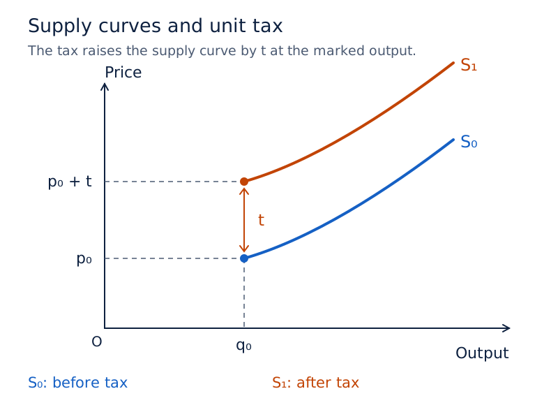
Price is on the vertical axis and output on the horizontal axis. S₁ lies above and to the left of S₀. At q₀, the marked price changes from p₀ to p₀ + t.
Drawn by One Young India.
At an unchanged market price, the tax reduces the firm's supply. Do not interpret the upward displacement of the curve as an increase in supply; its equivalent leftward displacement shows the decrease.
What are the exceptions and qualifications to the law of supply?
The law assumes that sellers can respond to a price change while other relevant conditions remain unchanged. Some cases limit that response; others involve changes in expectations or a choice between work and leisure. Explain the mechanism instead of merely naming an exception.
When is the available quantity fixed?
For a rare good whose existing quantity cannot be reproduced, a higher price cannot create additional originals. Its available quantity may remain fixed. This is a limit to increasing supply, rather than a claim that supply necessarily falls as price rises.
With perishable goods, which deteriorate if kept, sellers may have little scope to postpone sale. When goods cannot be stored and the selling period is very short, the available quantity may have to be offered even at a lower price.
The time condition matters. These cases should not be turned into a statement that every perishable commodity has the same supply response in every period. A restriction on the current stock is different from the possibility of changing future production.
How can expectations or labour supply alter the response?
If sellers expect a further price rise, they may withhold stock instead of offering more immediately at the higher current price. Expectations have changed, so the other-things-equal assumption behind the simple law no longer holds.
Labour supply means the amount of work people are willing to offer. At sufficiently high wages, a worker may prefer more leisure, meaning time outside paid work, and reduce working hours. The resulting labour-supply curve may bend backwards.
This labour case is conditional, not universal. Higher wages do not necessarily reduce hours at all wage levels or for all workers. It also concerns the supply of labour services rather than the ordinary output supply of a competitive firm.
Note: A supply curve shifting because technology or input prices change is not, by itself, a refutation of the law. The law isolates the effect of the commodity's own price while those other conditions remain constant.
How is market supply derived from individual supply?
Market supply is the total quantity offered by all firms at a given market price. Derive it by adding individual quantities at that same price. Do not add the prices faced by different firms.
Let S₁(P) and S₂(P) denote the quantities supplied by firms 1 and 2 at price P, and let Sₘ(P) denote market supply. Then Sₘ(P) = S₁(P) + S₂(P). The notation in brackets means that each quantity depends on P.
Why is the summation horizontal?
On the graph, price is measured vertically and output horizontally. Holding price fixed means staying at one vertical level. Adding the firms' quantities therefore adds horizontal distances. This is horizontal summation.
In the figure below, S₁ and S₂ label the individual supply curves and Sₘ labels the market curve. The prices p₁ and p₂ mark their different starting thresholds. At the higher price p₃, q₃ and q₄ are the two firms' outputs, and q₅ is their combined output.
What the figure shows
The market supply curve
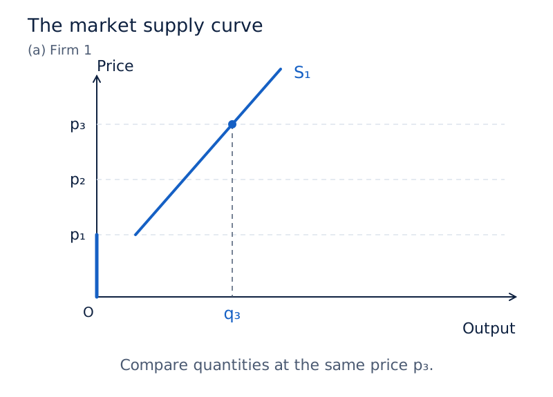
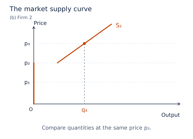
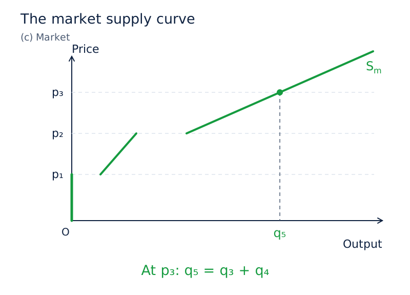
Three panels show firm 1, firm 2 and the market. At the common price p₃, the quantities q₃ and q₄ in the first two panels are added to give q₅ in the market panel.
Drawn by One Young India.
Worked example 2. Firm 1 supplies zero below price 10 and supplies P − 10 when P is at least 10. Firm 2 supplies zero below price 15 and supplies P − 15 when P is at least 15. Derive their combined supply.
Answer: Market supply is zero when P < 10. It equals P − 10 when 10 ≤ P < 15. When P ≥ 15, it equals (P − 10) + (P − 15) = 2P − 25.
At price 15, firm 2's stated formula gives zero; it becomes positive above 15. Checking the boundary values prevents an incorrect assertion that every firm necessarily supplies a positive amount at its threshold.
The derived market curve assumes a fixed number of firms. Entry of additional firms shifts market supply rightward, while a decrease in their number shifts it leftward. These changes alter the total supplied at a given price.
What is price elasticity of supply, and what are its degrees?
Price elasticity of supply measures the responsiveness of quantity supplied to a change in the commodity's price. The law of supply indicates the direction of a response; elasticity measures its proportionate size.
Let eₛ denote price elasticity of supply. Then eₛ = percentage change in quantity supplied ÷ percentage change in price. Compare percentage changes, not the absolute number of extra units with the absolute number of extra rupees.
Elasticity is independent of units. Expressing quantity in a different physical unit does not change the percentage response if both initial and final quantities are converted consistently. Elasticity itself is a pure number, not a quantity of goods or rupees.
How are the degrees distinguished?
| Degree | Elasticity | Meaning |
|---|---|---|
| Perfectly inelastic | eₛ = 0 | Quantity does not respond to price |
| Relatively inelastic | 0 < eₛ < 1 | Quantity changes by a smaller percentage than price |
| Unitary elastic | eₛ = 1 | Quantity and price change by equal percentages |
| Relatively elastic | eₛ > 1 | Quantity changes by a larger percentage than price |
| Perfectly elastic | eₛ tends to infinity | A limiting case represented by a horizontal supply curve |
A vertical supply curve represents zero elasticity because quantity remains fixed as price varies. On an upward-sloping supply curve, quantity rises with price and elasticity is positive. A horizontal curve represents the limiting case of supply at one unchanged price.
The word “inelastic” does not mean “no change” unless elasticity is zero. With relatively inelastic supply, quantity does change, but its percentage change is smaller than the percentage change in price.
Similarly, unitary elasticity does not mean that one extra rupee causes one extra unit of supply. It means equality between the two percentage changes. Keeping this distinction clear avoids confusing the slope of a curve with its elasticity.
How is elasticity calculated by the percentage method?
Let P₁ be initial price, P₂ final price, Q₁ initial quantity supplied and Q₂ final quantity supplied. The symbol Δ means “change in”, so ΔP = P₂ − P₁ and ΔQ = Q₂ − Q₁.
Using the initial values as bases, eₛ = (ΔQ ÷ Q₁) ÷ (ΔP ÷ P₁). Equivalently, eₛ = (ΔQ ÷ ΔP) × (P₁ ÷ Q₁). Multiplying each fractional change by 100 gives percentages; the two factors of 100 cancel in their ratio.
How does the cricket-ball example work?
Worked example 3. In a perfectly competitive cricket-ball market, price rises from Rs 10 to Rs 30 per ball. Aggregate quantity supplied rises from 200 to 1,000 balls. Calculate price elasticity of supply using initial values.
Answer: ΔQ = 1,000 − 200 = 800 balls; ΔP = Rs 30 − Rs 10 = Rs 20. Quantity rises by (800 ÷ 200) × 100 = 400%. Price rises by (20 ÷ 10) × 100 = 200%. Thus eₛ = 400 ÷ 200 = 2.
Supply is relatively elastic over this change because the percentage increase in quantity is twice the percentage increase in price. The increase in quantity is 800 balls; 1,000 balls is the final quantity, not the change.
How can output be recovered from revenue?
Total revenue, denoted TR, is the firm's receipts from selling output. With P as price per unit and Q as quantity sold, TR = P × Q, so Q = TR ÷ P.
Worked example 4. A firm earns revenue of Rs 50 at a price of Rs 10. Price rises to Rs 15 and revenue becomes Rs 150. Calculate the price elasticity of the firm's supply.
Answer: Initial output = 50 ÷ 10 = 5 units. Final output = 150 ÷ 15 = 10 units. Quantity increases by 100%, and price increases by 50%. Therefore eₛ = 100 ÷ 50 = 2.
Revenue is not quantity. Recover quantities first; comparing the percentage change in revenue directly with the percentage change in price would answer a different question.
How can elasticity identify an unknown quantity?
Worked example 5. Price changes from Rs 5 to Rs 20, quantity supplied rises by 15 units, and eₛ = 0.5. Find initial and final quantities using the initial-value percentage method.
Answer: 0.5 = (15 ÷ Q₁) ÷ (15 ÷ 5) = 5 ÷ Q₁. Therefore Q₁ = 10 units, and Q₂ = 10 + 15 = 25 units. Quantity rises by 150%, compared with a 300% price rise.
Worked example 6. At Rs 10 a firm supplies 4 units. Price rises to Rs 30, and eₛ = 1.25. Find the new quantity using initial values.
Answer: Price rises by 200%. Quantity must rise by 1.25 × 200% = 250%. The increase is 250% of 4 = 10 units. Final supply is 4 + 10 = 14 units.
How does the geometric method measure elasticity?
The geometric method measures elasticity at a point on a straight-line supply curve using distances along the quantity axis. It shows why an upward slope alone does not tell us whether elasticity is greater than, equal to or less than one.
Which distances are compared?
Let S be the chosen point on the supply line, O the origin, and q₀ the point directly below S on the quantity axis. Let M be where the supply line, extended if necessary, meets that axis. The marked price at S is p₀.
The notation Mq₀ means the distance between M and q₀; Oq₀ means the distance from the origin to q₀. Then eₛ = Mq₀ ÷ Oq₀. Use the line's intercept, not merely its apparent steepness on the page.
- Select a point S on the straight-line supply curve.
- Drop a perpendicular from S to the quantity axis to locate q₀.
- Extend the supply line to meet that axis at M.
- Compare Mq₀ with Oq₀ to determine whether elasticity exceeds, equals or falls below one.
What the figure shows
Elasticity of straight-line supply curves
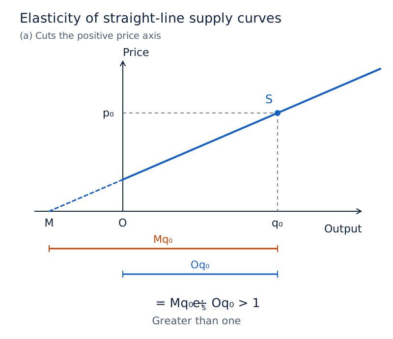
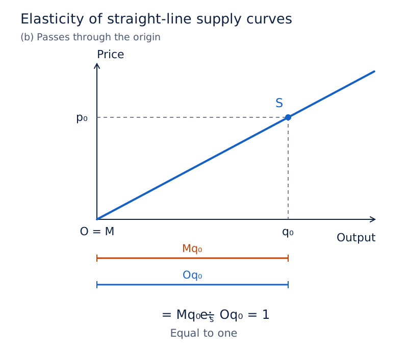
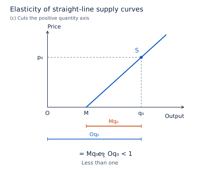
Three panels show price vertically and output horizontally. In panel (a), M is left of O. In panel (b), the line passes through O. In panel (c), M is right of O.
Drawn by One Young India.
| Position of straight supply line | Distance comparison | Elasticity |
|---|---|---|
| Cuts the positive price axis | Mq₀ exceeds Oq₀ | Greater than one |
| Passes through the origin | Mq₀ equals Oq₀ | Equal to one |
| Cuts the positive quantity axis | Mq₀ is less than Oq₀ | Less than one |
For a straight supply line through the origin, elasticity is one at every positive-output point, whatever the line's slope. At the origin itself, the displayed distance ratio has a zero denominator, so do not substitute zero into it.
The percentage method uses observed changes between stated prices and quantities. The geometric method uses the position of a point and the intercept of a straight line. Choose the method that matches the information supplied.
Glossary
- Supply — Quantity a seller is willing and able to offer at a stated price during a specified period.
- Stock — Total quantity of a commodity available with a seller at a particular time.
- Supply function — Relationship showing how quantity supplied depends on price and other determinants.
- Supply schedule — Table showing quantities supplied at different prices, with other determinants unchanged.
- Supply curve — Graph relating quantity supplied to price while holding other determinants constant.
- Ceteris paribus — Condition meaning that other relevant influences are held unchanged during an analysis.
- Marginal cost — Addition to total cost resulting from producing one extra unit of output.
- Extension of supply — Increase in quantity supplied caused by a rise in the commodity's own price.
- Contraction of supply — Decrease in quantity supplied caused by a fall in the commodity's own price.
- Increase in supply — Rightward shift allowing a larger quantity to be supplied at a given price.
- Unit tax — Tax imposed by the government per unit sale of a good.
- Market supply — Total quantity supplied by all firms at the same market price.
- Price elasticity of supply — Percentage change in quantity supplied divided by the percentage change in price.
- Horizontal summation — Addition of individual firms' quantities supplied at each common price to obtain market supply.
Common errors and misconceptions
- Misconception: Stock and supply are identical. Correct: Stock is the available quantity; supply identifies what is offered at a stated price during a period.
- Misconception: A higher selling price shifts the supply curve rightward. Correct: With other conditions unchanged, it causes a movement along the same curve.
- Misconception: Every upward displacement means increased supply. Correct: A unit tax shifts supply upward and leftward, reducing quantity at a given price.
- Misconception: Market supply adds firms' prices. Correct: It adds their quantities at each common price, which is horizontal summation.
- Misconception: A change in revenue is a change in quantity. Correct: Divide revenue by the corresponding price to recover quantity before calculating supply elasticity.
- Misconception: An elasticity below one means supply does not change. Correct: Positive elasticity below one means a smaller percentage quantity response than the percentage price change.
- Misconception: A straight supply line must have elasticity one. Correct: A straight line through the origin has unitary elasticity; its intercept determines the other cases.
Exam-style questions with model answers
Q1. Define supply and distinguish it from stock. [2 marks]
- Supply is the quantity a seller is willing and able to offer at a given price during a specified period.
- Stock is the total quantity available at a particular time; the whole stock need not be offered for sale.
Q2. Distinguish an extension of supply from an increase in supply in three respects. [3 marks]
- An extension follows a rise in the commodity's own price, with other determinants unchanged. An increase follows a change in another determinant, such as technological progress.
- An extension appears as an upward movement along the existing supply curve. An increase appears as a rightward shift of the curve.
- An extension compares quantities at different prices. An increase means that more can be supplied at the same price.
Q3. A technological improvement allows a firm to make the same output with fewer inputs. Explain its expected effect on marginal cost and supply, holding the market price unchanged. [4 marks]
- The improvement means that fewer productive resources are required to make the given output.
- It is expected to reduce marginal cost, which is the extra cost of producing another unit, at any output level.
- The marginal-cost curve shifts rightward or downward. Since the competitive firm's supply curve follows its relevant marginal-cost segment, supply shifts rightward.
- At the unchanged market price, the firm now supplies more output. This is an increase in supply, rather than a movement caused by a higher selling price.
Q4. A cricket-ball market supplies 200 balls at Rs 10 each and 1,000 balls at Rs 30 each. Calculate elasticity by the initial-value percentage method and interpret it. [5 marks]
- The initial quantity is 200 balls and the final quantity is 1,000, so the increase in quantity supplied is 800 balls.
- Using the initial quantity as the base, the percentage increase in quantity is (800 ÷ 200) × 100 = 400%.
- Price increases by Rs 20. Using the initial price of Rs 10, the percentage price increase is (20 ÷ 10) × 100 = 200%.
- Price elasticity of supply equals the percentage quantity change divided by the percentage price change, giving 400 ÷ 200 = 2.
- Supply is relatively elastic over this change: quantity supplied rises by twice the percentage rise in price. The elasticity value has no physical or currency unit.
Q5. At price P, firm 1 supplies zero for P < 10 and P − 10 for P ≥ 10. Firm 2 supplies zero for P < 15 and P − 15 for P ≥ 15. Derive market supply over the three price ranges. [3 marks]
- For P < 10, both firms supply zero, so market supply is zero. Adding supplies means adding quantities at the same price.
- For 10 ≤ P < 15, firm 2 still supplies zero. Market supply therefore equals firm 1's supply, P − 10.
- For P ≥ 15, add both stated expressions: (P − 10) + (P − 15) = 2P − 25. At P = 15, firm 2's contribution is zero.
Q6. Explain the geometric method for elasticity at a positive-output point S on a straight-line supply curve. Define the distances and explain all three intercept cases. [6 marks]
- Use price on the vertical axis and quantity on the horizontal axis. Mark the chosen positive-output point S on the straight supply line.
- Let O be the origin, q₀ the point directly below S on the quantity axis, and M the line's quantity-axis intercept, extending the line if necessary.
- Elasticity equals Mq₀ ÷ Oq₀, where each expression represents the distance between the two named points on the quantity axis.
- If the line cuts the positive price axis, M lies left of O. Mq₀ exceeds Oq₀, so elasticity exceeds one.
- If the line passes through O, the distances are equal. Their ratio is one, giving unitary elasticity.
- If the line cuts the positive quantity axis, M lies right of O. Mq₀ is smaller than Oq₀, so elasticity is below one.
Q7. A firm receives Rs 50 in revenue at price Rs 10, and Rs 150 in revenue at price Rs 15. Calculate supply elasticity using initial values. [4 marks]
- Quantity equals revenue divided by price. Initial quantity is therefore Rs 50 ÷ Rs 10 = 5 units.
- Final quantity is Rs 150 ÷ Rs 15 = 10 units. Quantity has increased by 5 units.
- The percentage quantity increase is (5 ÷ 5) × 100 = 100%; the percentage price increase is (5 ÷ 10) × 100 = 50%.
- Elasticity is 100 ÷ 50 = 2. Supply is relatively elastic because the percentage quantity response exceeds the percentage price change.
Q8. Explain two qualifications to the law of supply: non-reproducible rare goods and sellers expecting a further price rise. [4 marks]
- For a rare good that cannot be reproduced, the existing available quantity is fixed. A higher price cannot create additional originals.
- This limits a positive supply response. It does not imply that the quantity must fall whenever price rises.
- If sellers expect a further price rise, they may withhold stock now instead of offering more at the higher current price.
- The expectations case involves a change in another determinant. It therefore relaxes the other-things-equal condition under which the ordinary law is stated.
Key takeaways
- Supply connects willingness and ability to sell with a stated price and period; stock records the available quantity.
- The law of supply describes the response to the commodity's own price while other relevant determinants remain unchanged.
- Technological progress is expected to lower marginal cost, while higher input prices usually raise it alongside average cost.
- A price change causes movement along a supply curve; a change in another determinant shifts the curve.
- Market supply adds individual quantities at a common price, and changes in the number of firms shift market supply.
- Price elasticity compares percentage changes in quantity and price; it is independent of the units used.
- The cricket-ball example gives elasticity two because quantity increases by four hundred per cent and price by two hundred per cent.
- A straight supply line through the origin has unitary elasticity at positive-output points, regardless of its slope.
Test yourself
What information must accompany a quantity supplied?
State the commodity's price and the period to which the quantity supplied relates.
What does ceteris paribus mean?
It means that other relevant conditions remain unchanged while the effect of the selected variable is examined.
Does an increase in the commodity's own price shift its supply curve?
With other determinants unchanged, it causes an upward movement along the existing curve, called an extension of supply.
Why is market supply found by horizontal summation?
Quantities are measured horizontally and are added while the common price, measured vertically, is held fixed.
What happens to supply when a unit tax is imposed?
The firm's supply curve shifts leftward, so less output is supplied at a given market price.
What does a vertical supply curve imply about elasticity?
Elasticity is zero because quantity supplied remains unchanged when the price varies.
A straight supply line cuts the positive price axis. What is its elasticity at a positive-output point?
Elasticity exceeds one because its extended quantity-axis intercept makes the numerator distance exceed the distance from the origin.
Why must revenue be divided by price before using it in a supply-elasticity calculation?
Elasticity requires quantity changes, and dividing each revenue figure by its corresponding price recovers the quantities.
Try it
Decision-Making in Supply: Managing Inventory and Production
Step into the role of an agricultural producer to evaluate decisions regarding stock, supply, and crop allocation.
1You have 1,000 quintals of harvested wheat sitting in your storage warehouse. At the prevailing market price this month, you decide to offer only 200 quintals for sale. According to economic principles, how should these quantities be categorized?
Correct. Stock is a static concept representing total accumulated volume available at a point in time, whereas supply is a flow concept representing the specific quantity offered for sale at a given price over a specified time period. Stock can exceed supply when prices are insufficient to liquidate all inventory.
Incorrect. Supply cannot exceed stock, but stock can exceed supply when market prices do not induce the seller to offer the entire accumulated inventory for sale.
Incorrect. Stock is a static, non-flow concept (total volume available at a point in time), while supply is the flow concept qualified by price, quantity, and a time horizon.
2You cultivate both wheat and mustard as substitutes in production on the same agricultural plot. If the market price of mustard rises significantly while the price of wheat remains unchanged, what will happen to your supply of wheat?
Correct. When the price of a substitute in production (mustard) rises, wheat becomes relatively less profitable, prompting producers to reallocate land and resources toward mustard and causing the supply of wheat to decline.
Incorrect. Because mustard and wheat compete for the same resources as substitutes in production, an increase in mustard's price shifts resources away from wheat, reducing wheat supply.
Incorrect. According to the supply function, the price of related goods (Pr) is a determinant of supply; a rise in the price of a production substitute reduces the supply of the alternative good.
You have successfully applied the concepts of stock versus supply and the impact of prices of related goods in production decisions.