
Theory of Income and Employment | ISC Class 12 Economics Notes
On this page
Watch & explore
Start with a few high-quality watches, then dive into the notes below.
Try an idea before you read. Step into the shoes of an economic advisor and apply Keynesian principles to stabilize a shifting economy. Explore →

Learnacy Labs Try it hands-on: open the Macroeconomics lab
This note covers planned and actual demand, aggregate demand and supply, consumption and saving, average and marginal propensities, investment, equilibrium income, the investment multiplier, full employment, excess demand, deficient demand, and fiscal and monetary measures for correcting demand imbalances.
What determines income and employment in the short run?
What does the model hold constant?
The Keynesian model explains how expenditure influences output, income and employment. Its simple short-run version assumes a fixed price level and a constant interest rate. It concentrates on how much firms produce when the demand for their goods changes.
The assumption of ceteris paribus means that other things remain unchanged while one relationship is examined. Holding prices constant makes it possible to study changes in output separately from changes in the prices at which that output is sold.
This analysis initially assumes unused resources, including labour, machinery and buildings. Firms can expand production by using these resources more fully. The fixed-price assumption is therefore associated with an economy that has room to raise production.
How are production, income and jobs connected?
Production generates factor incomes. Labour receives wages, land receives rent, capital receives interest, and the entrepreneur receives profit. When additional goods are produced, the corresponding payments increase the incomes available for further expenditure.
Given the quantities of other factors, the level of output also determines employment. If demand supports a higher output, more labour can be employed. If spending is inadequate, some productive resources may remain unused even though the economy has reached an equilibrium.
Note: An equilibrium is a position with no tendency for income to change within the model. It does not, by itself, establish that all available factors of production are employed.
The central chain is therefore expenditure, production, factor income and further expenditure. Studying these links explains both why a demand shortage can persist and why an initial increase in investment can produce a larger eventual increase in income.
How do planned demand, actual demand and effective demand differ?
What do ex ante and ex post mean?
Ex ante describes a planned value. Consumption plans express what households intend to spend, while investment plans express what firms intend to add to capital or inventories. These plans need not match the amount that firms intend to produce.
Ex post describes a realised or actual value after economic activity has occurred. Unexpected sales can cause actual inventory investment to differ from planned inventory investment. The difference does not mean that the producer originally intended the actual result.
| Basis | Ex ante | Ex post |
|---|---|---|
| Meaning | Intended or planned amount | Realised or actual amount |
| Investment | Planned additions to capital and inventories | Actual additions, including unplanned inventory changes |
| Role in equilibrium | Plans must be mutually consistent | Accounting totals include what actually occurred |
Worked example 1. A producer plans to add Rs 100 of goods to inventory. Unexpected additional sales use Rs 30 of that planned addition. Find planned and actual inventory investment.
Answer: Planned inventory investment is Rs 100. Actual inventory investment is Rs 100 − Rs 30 = Rs 70. The unexpected sales make actual investment Rs 30 lower than planned investment.
What is effective demand?
Effective demand concerns the demand actually realised in expenditure and, in equilibrium analysis, the demand that sustains the equilibrium level of output. At the equilibrium point, planned aggregate demand equals aggregate supply.
The effective demand principle states that, with prices fixed and output able to respond, aggregate demand determines aggregate output. It explains the level at which production settles. Distinguish this equilibrium argument from the mere observation that actual expenditure has already taken place.
Actual output and actual expenditure remain equal in the two-sector accounting framework because unsold production counts as inventory investment. Planned spending can still fall short of output. That shortfall leads to unintended stock accumulation and gives producers a reason to change production.
What are the components of aggregate demand?
How does the sector coverage change the expression?
Aggregate demand is total planned expenditure on final goods and services at a given income level. In the simple two-sector model, households and firms provide the two sources of demand. Households consume goods and services, while firms undertake investment.
The two-sector expression is AD = C + I. Here C is planned consumption and I is planned investment. The model excludes government and foreign trade while deriving its basic income and multiplier results.
Including government adds its purchases of final goods and services, G. Including foreign trade adds demand from abroad, X, and subtracts spending on imports, M. The expenditure expression for domestic output is then AD = C + I + G + (X − M).
| Component | Meaning | Role in demand for domestic output |
|---|---|---|
| C | Household consumption expenditure | A source of spending on final goods and services |
| I | Investment expenditure | Additions to capital and changes in inventories |
| G | Government purchases | Public expenditure on final goods and services |
| X − M | Net exports | Exports add foreign demand; imports remove spending on foreign output |
Why must imports be subtracted?
Some expenditure by domestic buyers falls on goods produced abroad. Counting that expenditure as demand for domestic production would overstate demand for the country's own output. Imports are subtracted for this reason, while exports represent foreign purchases of domestic goods.
Net exports are positive when exports exceed imports and negative when imports exceed exports. Their inclusion changes the coverage of the model. Do not add foreign trade to a numerical problem that explicitly asks for the simple two-sector result.
Taxes also influence demand, but they are not an additional expenditure component. They affect households' disposable income and consequently their consumption. Government purchases influence demand directly; taxes influence it through the income available to households.
How does the consumption function relate spending to income?
What are autonomous and induced consumption?
A consumption function expresses the relationship between consumption expenditure and income. The simple linear function divides consumption into an income-independent component and a component that varies with income. Write it as C = C₀ + cY.
Here C₀ denotes autonomous consumption, c denotes the marginal propensity to consume, and Y denotes income. The term cY is induced consumption. Even when current income is zero, autonomous consumption remains positive in this model.
A constant c means that equal increases in income cause equal increases in consumption. It does not mean that total consumption stays constant. The consumption line rises because the induced component increases as income increases.
What the figure shows
Consumption function
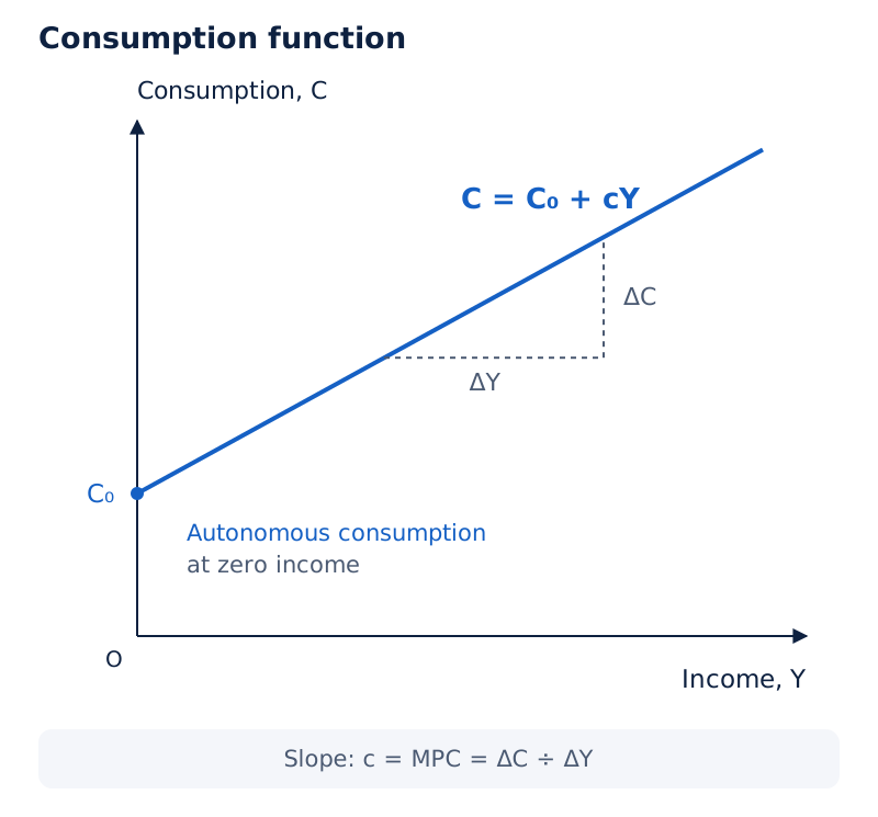
Income Y is on the horizontal axis and consumption C on the vertical axis. The rising straight line begins above the origin. Its vertical intercept represents autonomous consumption, and its slope represents the marginal propensity to consume.
Drawn by One Young India.
How can a function be interpreted numerically?
Worked example 2. Imagenia has the consumption function C = 100 + 0.8Y. Find autonomous consumption and the increase in consumption when income rises by Rs 100.
Answer: Autonomous consumption is Rs 100 and MPC is 0.8. The change in consumption is 0.8 × Rs 100 = Rs 80. The Rs 100 intercept is a level of consumption, not the increase caused by the additional income.
The intercept and slope describe different features. Changing autonomous consumption shifts the line vertically without changing its slope. Changing c alters the slope and therefore changes how strongly consumption responds to income.
When government taxes are introduced, consumption depends on disposable income. With lump-sum taxes T and no transfers, disposable income is Y − T. The corresponding consumption expression is C = C₀ + c(Y − T), making the link between taxation and spending explicit.
How are consumption and saving propensities calculated?
How do average and marginal ratios differ?
Saving is the part of income not consumed. The relationship is S = Y − C. Substituting the linear consumption function gives S = −C₀ + (1 − c)Y. Saving increases with income when the marginal propensity to save is positive.
An average propensity relates the total amount consumed or saved to total income. A marginal propensity relates a change in consumption or saving to the change in income that accompanies it. The symbol Δ means a change.
| Ratio | Formula | Interpretation |
|---|---|---|
| APC | C ÷ Y | Consumption per unit of total income |
| APS | S ÷ Y | Saving per unit of total income |
| MPC | ΔC ÷ ΔY | Extra consumption per unit of extra income |
| MPS | ΔS ÷ ΔY | Extra saving per unit of extra income |
Which relationships follow from the income identity?
Since Y = C + S, dividing by non-zero income gives APC + APS = 1. Similarly, dividing ΔY = ΔC + ΔS by a non-zero change in income gives MPC + MPS = 1. Therefore, MPS = 1 − MPC.
In the simple model, MPC lies between zero and one, inclusive. At zero, consumption does not respond to an income increase. At one, all additional income is consumed. Between these values, additional income is divided between consumption and saving.
With positive autonomous consumption, APC can exceed one at low income, and saving is then negative. At the break-even income, consumption equals income and saving is zero. At zero income, APC and APS cannot be calculated because their denominator is zero.
Worked example 3. Consumption is C = 40 + 0.8Y and income is 250 units. Calculate consumption, saving, APC, APS, MPC and MPS.
Answer: C = 40 + 0.8 × 250 = 240 units; S = 250 − 240 = 10 units. APC = 240 ÷ 250 = 0.96 and APS = 10 ÷ 250 = 0.04. MPC = 0.8 and MPS = 0.2.
Notice that APC differs from MPC in this example. The first uses total consumption, including autonomous consumption. The second measures the response to an income change. Replacing one ratio with the other would give an incorrect multiplier.
How do investment and aggregate supply enter the model?
What does autonomous investment mean?
Investment includes additions to physical capital and changes in producers' inventories. Machines, buildings and roads add to productive capacity. Inventories are stocks of output held by firms; an increase or decrease in them is inventory investment.
Capital goods provide services over time. They are final goods rather than intermediate goods used up in current production. This distinction keeps investment expenditure separate from the purchase of raw materials consumed during production.
The simple model treats planned investment as autonomous investment, written I = I₀. It is independent of current income, so its graph is horizontal. This is a modelling assumption, not a claim that investment can never change.
Credit availability and interest rates can influence investment decisions. Easier credit can encourage investment, while a higher interest rate raises the cost of funds and can discourage it. A change in autonomous investment shifts the aggregate demand schedule.
How is aggregate supply represented?
In the income-expenditure diagram, aggregate supply is represented by output or income Y. A 45° line shows equal values on the two axes. At each point on this line, the value of output supplied equals the corresponding income.
What the figure shows
Aggregate supply in the income-expenditure diagram
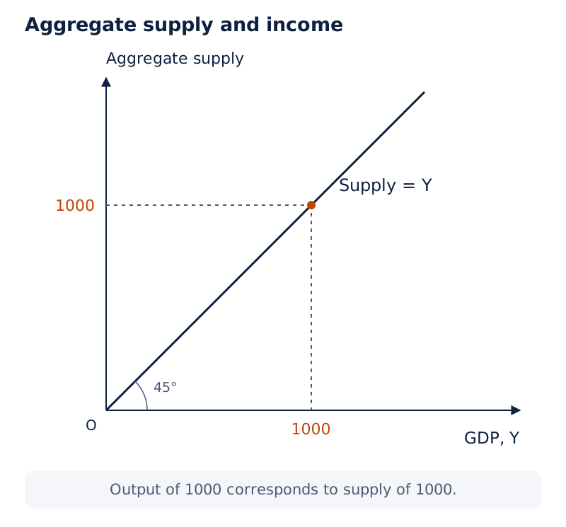
GDP, Y is on the horizontal axis and aggregate supply on the vertical axis. A straight line rises from the origin at 45°. The marked output of 1000 corresponds to an equal value of supply.
Drawn by One Young India.
The diagram measures income and expenditure values on comparable scales. It does not put the general price level on the vertical axis. A 45° supply line here therefore has a different meaning from a price-output supply curve.
Adding constant investment vertically to consumption produces an AD line parallel to the consumption line. Its intercept is C₀ + I₀ and its slope remains c, because the investment component does not vary with income in this model.
How is equilibrium income found by demand and supply or saving and investment?
How does the AD-AS method work?
Equilibrium income occurs where planned aggregate demand equals planned output. In the two-sector model, the condition is Y = C + I. Substitute C = C₀ + cY and I = I₀ to obtain the equilibrium value algebraically.
- Write the planned expenditure expression: AD = C₀ + cY + I₀.
- Set output equal to planned expenditure: Y = C₀ + cY + I₀.
- Move induced consumption to the left: Y − cY = C₀ + I₀.
- Factor and divide: Y(1 − c) = C₀ + I₀, so Y = (C₀ + I₀) ÷ (1 − c).
Writing A = C₀ + I₀ gives Y = A ÷ (1 − c). This finite solution requires c to be below one. Autonomous expenditure and the marginal propensity to consume jointly determine the equilibrium level.
What the figure shows
Equilibrium income
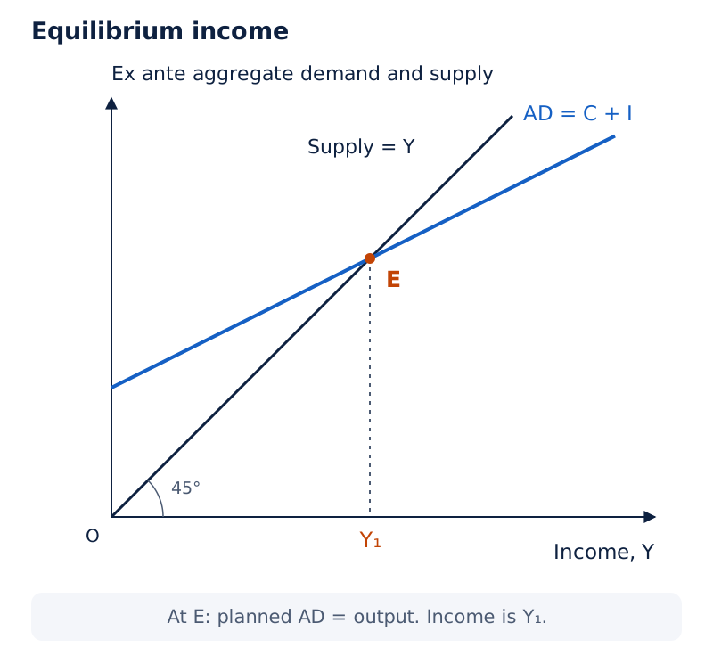
The horizontal axis is Y and the vertical axis measures ex ante aggregate demand and supply. The rising demand line crosses the 45° line at E. A dotted vertical line from E identifies equilibrium income Y₁.
Drawn by One Young India.
Why is saving equal to planned investment at equilibrium?
Starting from Y = C + I, subtract C from each side. Since Y − C = S, the same condition becomes S = I. Thus, the saving-investment approach and the demand-supply approach identify the same two-sector equilibrium.
Worked example 4. In a two-sector economy, C = 40 + 0.8Y and autonomous investment is 10 units. Find equilibrium income and verify saving equals investment.
Answer: Y = (40 + 10) ÷ (1 − 0.8) = 250 units. Consumption is 40 + 0.8 × 250 = 240 units. Saving is 250 − 240 = 10 units, equal to planned investment.
The equality refers to planned saving and investment when identifying equilibrium. Actual saving and actual investment also satisfy the accounting identity, but actual investment includes unintended stock changes. That accounting equality alone cannot establish that production plans are in balance.
How do firms adjust when planned demand differs from output?
What happens when demand is too low?
If planned demand is below output, firms cannot sell all the goods they intended to sell. Stocks accumulate beyond their plans. This unintended inventory investment signals that production exceeds the expenditure currently supported by households and firms.
- Planned spending falls short of the current value of output.
- Unsold output causes an unintended increase in inventories.
- Producers respond by reducing output in subsequent production rounds.
- Lower production reduces factor income and induced consumption until a consistent equilibrium is reached.
If planned demand exceeds output, sales draw down inventories more than firms intended. With unused resources available, firms have a reason to expand production. Additional production raises incomes and allows demand and output to adjust towards equality.
How can a numerical question identify disequilibrium?
Worked example 5. Total autonomous consumption and investment expenditure is Rs 50 crore, MPS is 0.2, and income is Rs 4,000 crore. Calculate planned aggregate demand and decide whether the economy is in equilibrium.
Answer: MPC = 1 − 0.2 = 0.8. AD = 50 + 0.8 × 4,000 = Rs 3,250 crore. Output exceeds planned demand by Rs 750 crore. The economy is not in equilibrium; inventories accumulate unintentionally and firms have a reason to reduce production.
Compare AD with Y after calculating demand. Reporting the spending total alone leaves the equilibrium question unanswered. The direction of the inequality identifies whether there is unintended stock accumulation or an unintended reduction in stocks.
This comparison diagnoses disequilibrium at a stated income level. To diagnose deficient or excess demand relative to full employment, the full-employment benchmark is also needed. The economy's current output must not be silently treated as full-employment output.
How does the investment multiplier increase equilibrium income?
What is the multiplier and how does it work?
The investment multiplier is the ratio of the total change in equilibrium income to the initial change in autonomous investment. In the simple two-sector model, k = ΔY ÷ ΔI = 1 ÷ (1 − MPC) = 1 ÷ MPS.
An investment increase creates demand for additional output. Producing that output generates incomes for the factors involved. Households consume a fraction of this extra income, creating further demand, further production and further income in successive rounds.
- An autonomous investment increase starts the process by increasing planned spending.
- Firms produce additional output and make additional factor payments.
- Income recipients spend the MPC fraction of their additional income.
- This induced consumption creates another round of output and income, continuing with successively smaller additions when MPC is below one.
Worked example 6. Initially C = 40 + 0.8Y and investment is 10 units. Investment rises to 20 units, while the consumption function is unchanged. Find the multiplier and the new equilibrium income.
Answer: k = 1 ÷ (1 − 0.8) = 5. Investment rises by 10 units, so income rises by 5 × 10 = 50 units. Initial income is 250 units and new income is 300 units.
| Round | Extra consumption demand | Extra output and income |
|---|---|---|
| First | 0; the initial increase is investment | 10 units |
| Second | 0.8 × 10 = 8 units | 8 units |
| Third | 0.8² × 10 = 6.4 units | 6.4 units |
| Fourth | 0.8³ × 10 = 5.12 units | 5.12 units |
What does the multiplier diagram show?
What the figure shows
Multiplier effect of higher investment
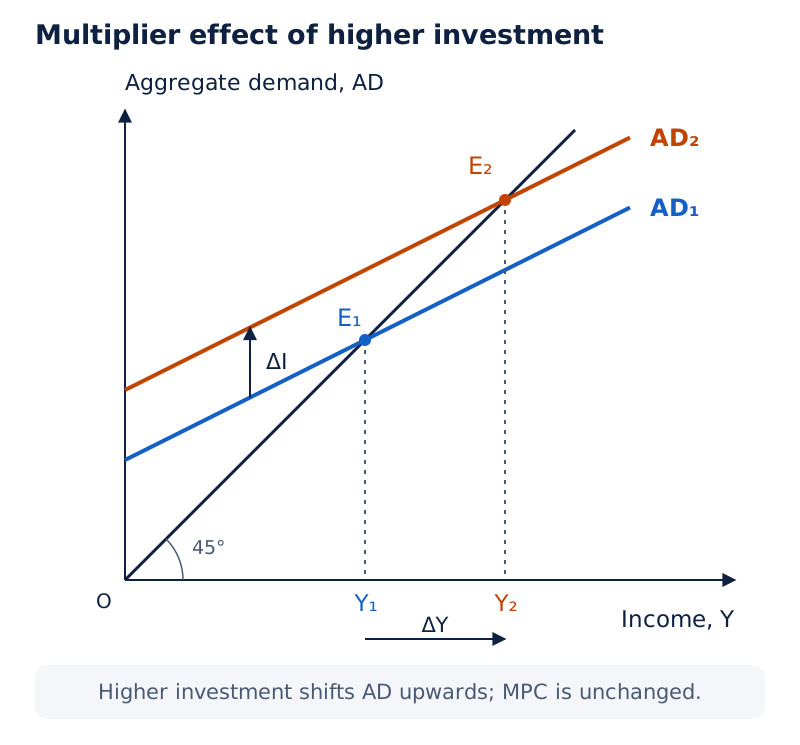
Income Y is on the horizontal axis and AD on the vertical axis. AD₂ lies parallel above AD₁. Their intersections with the 45° line are E₂ and E₁ respectively, with the new equilibrium farther to the right.
Drawn by One Young India.
The initial vertical rise in planned spending starts an adjustment that produces a larger horizontal increase in equilibrium income. The slope remains unchanged because MPC is unchanged. A shift caused by higher autonomous investment must not be drawn as a change in slope.
A higher MPC produces a larger multiplier because more of each income addition is spent again. A higher MPS produces a smaller multiplier. The formula describes a fixed-price economy with scope to expand output, rather than an unlimited ability to increase real production beyond capacity.
How do full employment, deficient demand and excess demand differ?
Why can equilibrium involve unemployment?
Full-employment income is the income level at which all factors of production are fully employed. The output associated with it provides a benchmark for judging whether aggregate demand is adequate to use the economy's available productive resources.
Equilibrium merely requires planned demand to equal output. These two quantities can be equal at an income below the full-employment level. Firms then have no demand-based incentive to produce more, although some resources remain unemployed.
How are the two demand problems identified?
Deficient demand occurs when demand is insufficient to purchase the output that would be produced at full employment. The economy settles below full-employment output in the simple model. Inadequate demand leaves resources unemployed and can exert downward pressure on prices over time.
Excess demand occurs when demand exceeds the output available at full employment. Demand cannot be met through the same expansion of real output assumed when resources are idle. It therefore generates upward pressure on prices.
| Comparison | Deficient demand | Excess demand |
|---|---|---|
| Full-employment benchmark | Demand falls short of full-employment output | Demand exceeds full-employment output |
| Main problem | Unused resources and unemployment | Inflationary pressure |
| Policy direction | Raise aggregate demand | Reduce aggregate demand |
The demand shortfall at full-employment income is called a deflationary gap; the excess is called an inflationary gap. Measure the expenditure gap at the full-employment level, rather than confusing it with the horizontal difference between two income levels.
Diagram
Demand gaps at full employment
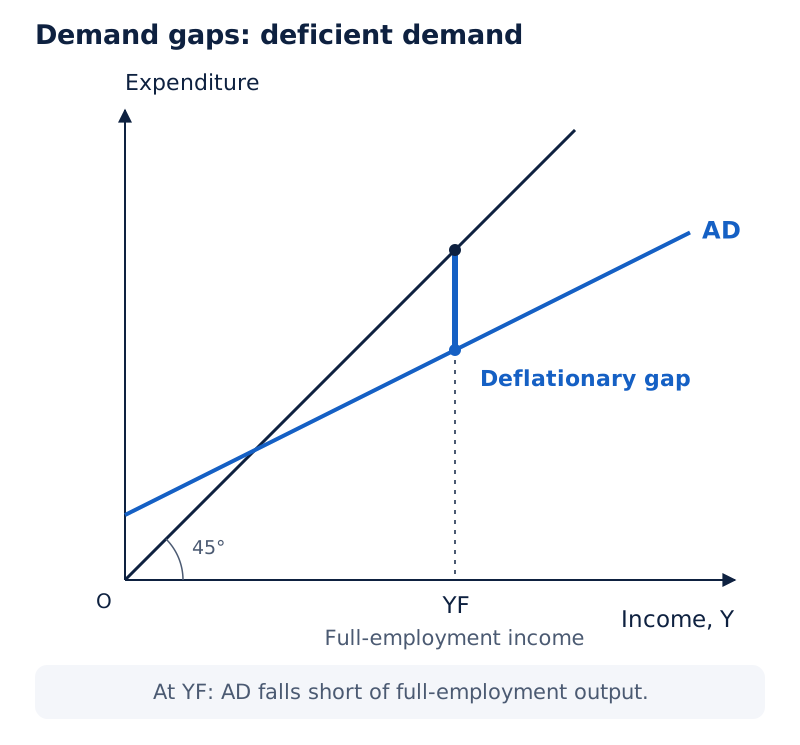
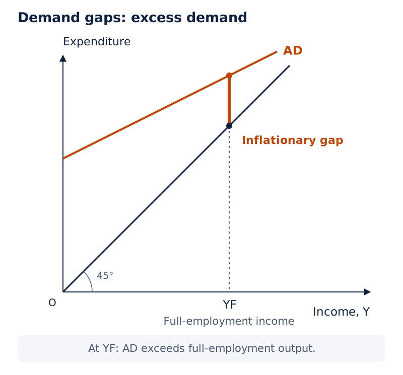
Draw income horizontally, expenditure vertically and a 45° reference line. Mark full-employment income YF. At YF, show an AD line below the reference line for deficient demand and above it for excess demand. Label the respective vertical gaps.
Drawn by One Young India.
A gap diagram asks whether demand supports full employment. A general inventory-adjustment diagram asks whether demand matches current output. Keeping these questions separate prevents the incorrect conclusion that every temporary demand imbalance is a full-employment demand gap.
How can fiscal policy correct demand imbalances?
How does government spending change demand?
Fiscal policy uses government expenditure and taxation to influence economic activity. Its stabilisation role is to counter fluctuations in income, employment and prices. The appropriate direction depends on whether total spending is insufficient or excessive.
During deficient demand, government can increase purchases of goods and services. These purchases add directly to aggregate demand. Firms respond to additional orders by producing more, and the resulting factor incomes support further consumption through the multiplier mechanism.
During excess demand, reducing government purchases restrains expenditure. The purpose is to reduce pressure on available output. The same instrument therefore works in opposite directions depending on the demand problem being addressed.
How do taxes and transfers affect consumption?
A reduction in taxes raises disposable income at a given gross income. Households consume a fraction of the additional disposable income, increasing demand. A tax increase has the opposite effect and can help restrain excess demand.
Transfer payments affect household disposable income without being government purchases of current goods and services. Higher transfers support consumption; lower transfers restrain it. Their initial effect on spending depends on the fraction of disposable income households consume.
| Instrument | To address deficient demand | To address excess demand |
|---|---|---|
| Government purchases | Increase purchases to add directly to demand | Reduce purchases to restrain demand |
| Taxes | Reduce taxes to support disposable income | Increase taxes to restrain disposable income |
| Transfers | Increase transfers to support household spending | Reduce transfers to restrain household spending |
Government spending and a tax reduction of the same amount do not have identical initial effects. Purchases enter aggregate demand directly. A tax reduction first raises disposable income, of which only the MPC fraction becomes additional consumption.
The policy explanation should therefore connect the instrument to expenditure and then to production or prices. Simply saying that a government should change taxes leaves the direction and mechanism unspecified. State whether demand needs to rise or fall and explain how the proposed change achieves that direction.
How can monetary policy influence demand and employment?
How do interest rates and credit matter?
Monetary policy influences money and credit conditions. In India, the Reserve Bank of India, or RBI, uses instruments affecting commercial banks and money supply. Credit availability and the cost of borrowing can influence investment, which is a component of aggregate demand.
To address deficient demand, easier credit conditions can encourage borrowing and investment. To restrain excess demand, tighter credit conditions can discourage expenditure financed through borrowing. The transmission works through spending decisions rather than adding government purchases directly.
A lower bank rate makes central-bank funds less expensive for commercial banks and can support monetary expansion. A higher rate works in the opposite direction. Lower borrowing costs can encourage firms to invest; higher costs can discourage investment.
How do reserves and open market operations work?
A lower cash reserve ratio permits banks to support more lending against a given reserve base. A higher ratio restricts lending capacity. Thus, reserve requirements can help influence credit and, through credit-financed spending, aggregate demand.
Through open market operations, the central bank buys or sells government bonds. Purchases add reserves to the banking system and expand money supply. Sales withdraw reserves and reduce money supply. These are opposite operations and must be matched to the policy objective.
| Instrument | Expansionary direction | Restrictive direction |
|---|---|---|
| Bank rate | Lower the rate | Raise the rate |
| Cash reserve ratio | Lower the required ratio | Raise the required ratio |
| Open market operations | Buy government bonds | Sell government bonds |
Moral suasion involves central-bank persuasion to encourage or discourage commercial-bank lending. It is a qualitative method. Reserve-ratio changes, bank-rate changes and open market operations are quantitative methods affecting the extent of money supply.
For a complete policy answer, identify the imbalance, choose the correct direction, and trace the effect through reserves or borrowing costs to investment and aggregate demand. When unused resources exist, stronger demand can support production and employment; at full employment, demand restraint addresses inflationary pressure.
Glossary
- Aggregate demand — Total planned expenditure on final goods and services at a given level of income.
- Aggregate supply — The value of output supplied, represented by income in the simple income-expenditure model.
- Ex ante — Describes a planned value of consumption, investment or output before its actual realisation.
- Ex post — Describes the realised value of an economic variable after the relevant activity has occurred.
- Effective demand — Demand realised in expenditure; at equilibrium, the demand sustaining the economy's level of output.
- Autonomous consumption — The component of consumption independent of current income, represented by the consumption function's intercept.
- Induced consumption — The component of consumption that varies with income according to the marginal propensity to consume.
- Marginal propensity to consume — The change in consumption divided by the corresponding change in income.
- Marginal propensity to save — The change in saving divided by the corresponding change in income.
- Average propensity to consume — Total consumption divided by total income, where income is non-zero.
- Average propensity to save — Total saving divided by total income, where income is non-zero.
- Investment multiplier — The ratio of the change in equilibrium income to the initial change in autonomous investment.
- Full-employment income — The income level associated with full employment of all factors of production.
- Deficient demand — A situation in which aggregate demand is insufficient to purchase full-employment output.
- Excess demand — A situation in which aggregate demand exceeds the output available at full employment.
Common errors and misconceptions
- Misconception: Ex ante and ex post investment are necessarily identical. Correct: Unexpected sales or unsold stocks can make actual inventory investment differ from planned investment.
- Misconception: APC and MPC measure the same ratio. Correct: APC uses total consumption and income; MPC uses changes in those quantities.
- Misconception: Autonomous investment can never change. Correct: It is independent of current income in the model, but other influences can change its level.
- Misconception: Equilibrium necessarily means full employment. Correct: Planned demand and output can be equal while productive resources remain unemployed.
- Misconception: The investment multiplier equals MPC. Correct: In the simple two-sector model, it equals 1 ÷ (1 − MPC), or 1 ÷ MPS.
- Misconception: Any demand shortfall proves a deflationary gap. Correct: A deflationary gap is measured against demand required at full-employment income.
- Misconception: Selling government bonds expands money supply. Correct: Central-bank sales withdraw reserves; purchases add reserves and support monetary expansion.
- Misconception: A tax cut and an equal increase in government purchases have identical initial effects. Correct: Purchases enter demand directly; a tax cut affects consumption through disposable income.
Exam-style questions with model answers
Q1. Define MPC and state its relationship with MPS. [2 marks]
- MPC is the change in consumption divided by the corresponding change in income: MPC = ΔC ÷ ΔY.
- Additional income is consumed or saved, so MPC + MPS = 1.
Q2. A producer plans to add Rs 100 to inventory, but unexpected extra sales reduce that addition by Rs 30. Calculate ex ante and ex post inventory investment. [2 marks]
- Ex ante inventory investment is the planned addition of Rs 100.
- Ex post inventory investment is the actual addition: Rs 100 − Rs 30 = Rs 70. Unexpected sales explain the difference.
Q3. Given C = 40 + 0.8Y and Y = 250 units, calculate consumption, saving, APC, APS, MPC and MPS. Explain why APC differs from MPC. [4 marks]
- Consumption is C = 40 + 0.8 × 250 = 240 units. Saving is S = Y − C = 250 − 240 = 10 units.
- APC = 240 ÷ 250 = 0.96, while APS = 10 ÷ 250 = 0.04. Their sum is one.
- MPC is the coefficient of income, 0.8. MPS = 1 − 0.8 = 0.2.
- APC includes autonomous consumption in total consumption. MPC measures the response of consumption to a change in income, so the ratios differ.
Q4. In a two-sector economy, C = 40 + 0.8Y and I = 10 units. Find equilibrium income and verify it by the saving-investment method. [4 marks]
- Equilibrium requires planned demand to equal output: Y = C + I = 40 + 0.8Y + 10.
- Rearranging gives 0.2Y = 50, so equilibrium income is 250 units.
- At this income, consumption is 40 + 0.8 × 250 = 240 units. Saving is 250 − 240 = 10 units.
- Planned saving therefore equals planned investment. Both the demand-supply method and the saving-investment method identify the same equilibrium.
Q5. Total autonomous expenditure is Rs 50 crore, MPS is 0.2 and current income is Rs 4,000 crore in a two-sector economy. Calculate AD and explain the direction of adjustment. [3 marks]
- MPC = 1 − MPS = 0.8. Planned AD = 50 + 0.8 × 4,000 = Rs 3,250 crore.
- Current output exceeds planned expenditure by Rs 750 crore, so the economy is not in equilibrium.
- Unsold output adds unintentionally to inventories. Firms have a reason to reduce production, lowering factor incomes and induced consumption as the adjustment towards equilibrium proceeds.
Q6. In a fixed-price two-sector economy with unused resources, C = 40 + 0.8Y and investment rises from 10 to 20 units. Calculate the multiplier and both equilibrium incomes. Explain the mechanism and the change in the AD diagram. [6 marks]
- The multiplier is k = 1 ÷ (1 − 0.8) = 5. Initial equilibrium income is (40 + 10) ÷ 0.2 = 250 units.
- Investment increases by 10 units. The resulting income increase is 5 × 10 = 50 units, giving a new equilibrium income of 300 units.
- The initial investment creates additional production and factor income. Households spend 0.8 of that income, generating another round of demand and production. Subsequent rounds add smaller amounts because some extra income is saved.
- On a diagram with Y horizontally and AD vertically, AD shifts parallel upwards. Its slope remains 0.8. The new intersection with the 45° line lies to the right, showing higher equilibrium income.
Q7. Explain why an economy can be in equilibrium below full employment. Describe two fiscal measures to correct deficient demand and their mechanisms. [5 marks]
- Equilibrium means planned aggregate demand equals output. This equality can occur below the output that would fully employ all factors, so equilibrium does not guarantee full employment.
- Deficient demand means spending is insufficient to purchase full-employment output. Firms have inadequate demand to justify using all available resources.
- Government can increase purchases of goods and services. This adds directly to demand, encouraging production and generating factor incomes that support further consumption.
- Government can reduce taxes. Disposable income rises, and households spend a fraction of the increase. Higher consumption raises aggregate demand and can support output and employment while resources remain unused.
Q8. An economy has aggregate demand above its full-employment output. Identify the problem and explain one fiscal and two monetary measures that can restrain it. [5 marks]
- The economy faces excess demand. Spending exceeds the output available at full employment, placing upward pressure on prices.
- The government can reduce purchases of goods and services. This directly reduces aggregate expenditure and helps restrain demand.
- The central bank can raise the cash reserve ratio. Banks must retain a larger reserve fraction, restricting their capacity to lend and thereby restraining credit-financed expenditure.
- The central bank can sell government bonds through open market operations. These sales withdraw reserves and reduce money supply. Tighter credit conditions can discourage investment expenditure, reducing aggregate demand and pressure on full-employment output.
Key takeaways
- Planned expenditure can differ from actual expenditure because unexpected sales create unintended inventory changes.
- In the two-sector model, aggregate demand consists of consumption and investment, and equilibrium requires Y = C + I.
- Average propensities use total income, while marginal propensities use income changes; each consumption-saving pair sums to one.
- Autonomous consumption determines the consumption function's intercept, while MPC determines its slope and response to additional income.
- Planned saving equals planned investment at the same income where planned aggregate demand equals aggregate supply.
- The investment multiplier equals one divided by MPS in the simple fixed-price two-sector model.
- Equilibrium can occur below full employment, leaving resources unused when aggregate demand is inadequate.
- Deficient demand calls for expansionary measures; excess demand calls for measures that restrain aggregate expenditure.
Test yourself
Why can actual investment differ from planned investment?
Unexpected sales or unsold output change inventories, creating an unplanned component of actual investment.
Why does adding autonomous investment leave the AD slope unchanged?
Autonomous investment adds the same amount at every income level, so AD retains the consumption function's slope.
How is MPS related to MPC?
MPS equals one minus MPC because additional income is divided between consumption and saving.
What signals firms to reduce production when planned demand is below output?
Unintended accumulation of unsold inventories signals that current production exceeds planned expenditure.
Why does an investment increase generate further rounds of income?
Additional production generates factor incomes, part of which is consumed, creating further demand and production.
Does equality of AD and output prove full employment?
No. Demand and output can be equal below the income that would fully employ all factors.
Why can a tax reduction increase aggregate demand?
It raises disposable income, allowing households to increase consumption according to their marginal propensity to consume.
Which open market operation can support an expansion of money supply?
A central-bank purchase of government bonds adds reserves to the banking system and supports monetary expansion.
Try it
Keynesian Economics in Action
Step into the shoes of an economic advisor and apply Keynesian principles to stabilize a shifting economy.
1You are monitoring a two-sector economy and notice a sudden shift in household behavior: total planned saving has begun to exceed total planned investment by firms. Based on Keynesian theory, what will be the immediate consequence of this imbalance?
Correct! The text states that when planned saving exceeds planned investment, households are hoarding money rather than spending. This drops Aggregate Demand, causing unsold inventory to pile up, which forces firms to cut production and lay off workers.
Incorrect. Inventories deplete when Aggregate Demand is greater than Aggregate Supply. When saving exceeds investment, people are spending less, meaning inventories will actually pile up, not deplete.
Incorrect. Effective Demand is the specific point where planned AD perfectly matches planned AS. An imbalance between saving and investment means the economy is not in equilibrium and employment must change to restore it.
2To combat the economic slowdown, a new initial investment is injected into the economy. You want this injection to generate the largest possible increase in final national income. Which condition would guarantee the largest multiplier effect?
Correct! The text explains that the size of the investment multiplier depends entirely on the MPC. The higher the MPC, the more people spend their extra income, creating a larger chain reaction of spending and income.
Incorrect. The text notes that if people save everything (MPS = 1), the multiplier is just 1, and the chain reaction stops immediately. A higher MPS actually shrinks the multiplier effect.
Great job! You successfully applied the concepts of Aggregate Demand, the S-I approach to equilibrium, and the Investment Multiplier to navigate macroeconomic shifts.