
Determination of Income and Employment | CBSE Class 12 Economics Notes
On this page
Watch & explore
Start with a few high-quality watches, then dive into the notes below.

This note covers planned and actual expenditure, consumption and saving, investment, aggregate demand, short-run income determination, equilibrium graphs, changes in autonomous expenditure, the multiplier mechanism, the paradox of thrift, employment, deficient demand and excess demand.
What assumptions explain income determination in this model?
Macroeconomic models are theoretical tools used to explain how economy-wide variables are determined. Such variables include national income, meaning total factor payments in the economy, the price level, the rate of interest and unemployment. Studying all their interactions at once is difficult, so a model begins with simplifying assumptions.
Ceteris paribus means other things remaining equal. When investigating one variable, the values of other variables are held constant. This helps isolate the relationship being studied before the analysis is extended to include further changes.
The income-determination model is based on the theory of John Maynard Keynes. It assumes fixed prices of final goods and a constant rate of interest. Final goods include goods for consumption and investment goods, such as machines.
Why can output change while prices remain fixed?
The starting assumption is that the economy has unused resources, including machinery, buildings and labour. Additional output can therefore be produced without increasing marginal cost, the cost of producing additional output. The price level need not change as production changes in this situation.
Holding prices fixed is also a simplifying assumption. The analysis first determines equilibrium with a fixed price level, then allows for the possibility of price changes at a later stage. It does not claim that prices remain fixed in every economic situation.
Aggregate output is the total output of final goods and services. Aggregate demand is planned total expenditure on final goods and services. Under the fixed-price assumptions, changes in this expenditure determine changes in output.
Definition: The effective demand principle means that aggregate output is determined solely by aggregate demand when supply can respond at the assumed constant price.
The analysis concentrates on a two-sector model, with households and firms providing consumption and investment demand. These assumptions must accompany the conclusions: a result about income in this model is not an unconditional statement about every economy.
How do ex ante and ex post values differ?
Ex ante means planned, while ex post means actual or realised. Consumption, investment and output can each be measured in either sense. A plan made for a period need not match the outcome recorded when that period ends.
Income determination requires the planned values of the components of demand. National income accounting, by contrast, records actual values. Confusing these two uses makes an accounting equality appear to prove equilibrium even when producers' and buyers' plans do not match.
How can actual investment differ from its plan?
Inventories are stocks of output that have been produced but remain unsold with a firm. Inventory investment is the change in these stocks. An increase is positive inventory investment; a depletion is negative inventory investment.
Worked example 1. A producer plans to add ₹100 worth of goods to her stock during the year. Unexpectedly high demand makes her sell ₹30 worth from that stock. Find planned and actual investment.
Answer: Planned investment is ₹100. Actual inventory addition is ₹100 − ₹30 = ₹70. Ex ante investment therefore exceeds ex post investment by ₹30 because unexpected sales reduce the planned stock addition.
| Basis | Ex ante | Ex post |
|---|---|---|
| Meaning | Planned value for the period | Actual value realised in the period |
| Inventory example | Planned addition of ₹100 | Actual addition of ₹70 |
| Demand and output | Plans coincide at equilibrium | Accounting includes unintended stock changes |
Planned inventory investment occurs when the firm deliberately decides to keep stocks. Unplanned inventory investment occurs when actual sales differ from expected sales, forcing stocks to rise or fall relative to the firm's plan.
Thus a difference between planned expenditure and planned output has a concrete counterpart: an unintended stock change. The producer's original plan and the resulting actual investment must be kept separate when explaining how an economy adjusts.
How does the consumption function relate spending to income?
The consumption function describes the relationship between household consumption expenditure and income. Household income is the most important determinant of consumption demand. The simplest function assumes that consumption changes at a constant rate when income changes.
Let C denote household consumption expenditure, Y income, C̄ autonomous consumption and c the marginal propensity to consume, meaning the change in consumption per unit change in income.
C = C̄ + cY
Autonomous consumption is independent of income. It explains why consumption can take place even when income is zero. The term cY is induced consumption, the part that depends on income. An increase in income raises this component according to the value of c.
What does the marginal propensity to consume measure?
Marginal propensity to consume (MPC) measures the change in consumption divided by the change in income. The symbol Δ means change, so ΔC is the change in consumption and ΔY is the change in income.
MPC = ΔC/ΔY
Generally, MPC lies between 0 and 1, inclusive of both values. At 0, consumption does not change when income changes. At 1, the entire change in income goes into consumption. Between these values, part of additional income is consumed.
Worked example 2. Imagenia has the consumption function C = 100 + 0.8Y, with monetary values in rupees. Identify autonomous consumption and find the consumption increase when income rises by ₹100.
Answer: Autonomous consumption is ₹100 and MPC is 0.8. The increase in consumption is 0.8 × ₹100 = ₹80. Even at zero income, the function gives consumption of ₹100.
The consumption function separates the level of spending independent of income from the response to income. The number 100 in Imagenia's function describes the former; 0.8 describes the latter. They therefore answer different questions about household expenditure.
How are consumption and saving propensities related?
Saving is the part of income that is not consumed. Let S represent saving. Subtracting consumption from income gives the saving identity, which connects the two uses of income.
S = Y − C
Marginal propensity to save (MPS) is the change in saving per unit change in income. Denote it by s. With ΔS meaning the change in saving, its formula is MPS = ΔS/ΔY.
Why do the marginal propensities add to one?
- Begin with saving as income minus consumption: S = Y − C.
- For changes in the variables, ΔS = ΔY − ΔC.
- Divide throughout by the change in income: ΔS/ΔY = 1 − ΔC/ΔY.
- Recognise the two ratios as MPS and MPC, giving s = 1 − c.
MPS + MPC = 1
The extra income is divided between extra consumption and extra saving. A greater share consumed therefore means a smaller share saved. In the consumption example with MPC of 0.8, MPS is 1 − 0.8 = 0.2.
Average propensity to consume (APC) is consumption per unit of income. Average propensity to save (APS) is saving per unit of income. These average ratios use total values, whereas marginal ratios use changes in those values.
| Measure | Formula | Meaning |
|---|---|---|
| MPC | ΔC/ΔY | Consumption change per unit income change |
| MPS | ΔS/ΔY | Saving change per unit income change |
| APC | C/Y | Consumption per unit of income |
| APS | S/Y | Saving per unit of income |
To choose the correct ratio, first identify whether the question supplies total income and expenditure or changes in them. An average describes how an existing income is used; a marginal propensity describes the response when income changes.
What is investment, and why is it autonomous here?
Investment means additions to physical capital and changes in a producer's inventories. Physical capital includes machines, buildings and roads that add to the future productive capacity of the economy. Investment therefore includes both capital additions and inventory changes.
Investment goods are final goods. A machine produced during a year is not used up like a raw material in producing another good during that year. It supplies services over a number of years, which distinguishes it from an intermediate good.
Let I denote planned investment and Ī the positive constant representing autonomous investment. The model assumes that firms plan to invest the same amount every year.
I = Ī
Does autonomous mean unaffected by every influence?
Autonomous investment means investment is independent of income in this analysis. It does not mean investment can never change. Variables other than income can influence it, even though they are held constant when a particular investment function is drawn.
Investment decisions depend, to a large extent, on the market rate of interest. The interest rate is the cost of investible funds. At higher interest rates, firms tend to lower investment. Easy availability of credit encourages investment.
It is therefore possible to compare one autonomous investment level with another. Each level is independent of income, but a change in the conditions governing investment can move the economy from one investment schedule to another.
What the figure shows
Autonomous investment
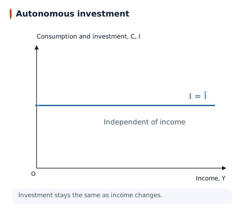
Income Y is on the horizontal axis. The vertical axis is labelled C, I for consumption and investment. The investment line, labelled I = Ī, is horizontal above the income axis.
Drawn by One Young India. See Fig. 4.3 in your NCERT textbook
The horizontal shape shows that investment remains the same at different income levels within this model. The height represents the given investment amount. A horizontal investment line therefore expresses an assumption about dependence on income, rather than a claim that firms face no changing conditions.
How is aggregate demand formed in the two-sector model?
In the two-sector economy, planned final demand comes from consumption and investment. Let AD denote aggregate demand. Combining the consumption function with autonomous investment gives the demand planned at each level of income.
AD = C + I
Substitution gives AD = C̄ + Ī + cY. Define Ā as total autonomous expenditure, equal to C̄ + Ī. The same demand function can then be written in a shorter form.
AD = Ā + cY
Autonomous consumption, representing subsistence consumption, remains more or less stable over time. Autonomous investment has been observed to undergo periodic fluctuations. Combining them in one symbol simplifies the equation without implying that they behave identically.
What do the intercept and slope represent?
An intercept is the value where a line meets the vertical axis, when the horizontal-axis variable is zero. A line's slope measures the vertical change associated with a unit horizontal change. For consumption, the intercept is C̄ and the slope is c.
What the figure shows
Consumption function
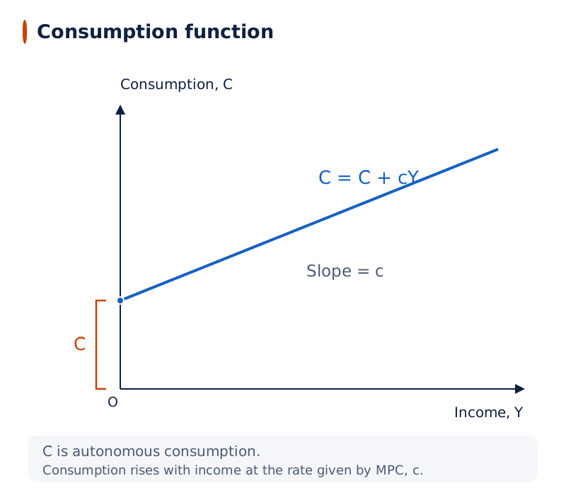
The upward-sloping line is labelled C = C̄ + cY. Consumption C is on the vertical axis and income Y on the horizontal axis. A bracket marks the positive vertical intercept C̄.
Drawn by One Young India. See Fig. 4.2 in your NCERT textbook
Adding autonomous investment to consumption raises demand by the same amount at each income level. The aggregate demand line is therefore parallel to the consumption line. Its intercept is C̄ + Ī, while its slope remains c.
What the figure shows
Building aggregate demand
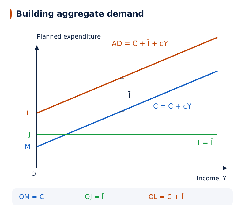
The figure shows a horizontal investment line and two parallel upward-sloping lines for consumption and aggregate demand. With O as the origin, M, J and L mark their vertical intercepts: OM = C̄, OJ = Ī and OL = C̄ + Ī.
Drawn by One Young India. See Fig. 4.4 in your NCERT textbook
Vertical addition means adding the consumption and investment amounts at the same income. The resulting line records ex ante demand, not necessarily expenditure that has already occurred or an equilibrium level of production.
How are short-run equilibrium income and output determined?
Aggregate supply is the output of final goods and services supplied in the economy. Gross domestic product (GDP) measures this aggregate output. With no government imposing indirect taxes or subsidies in the simplified model, Y is used for GDP or national income interchangeably.
Equilibrium in the final goods market occurs when planned aggregate demand equals planned aggregate supply. Plans made by suppliers then match the plans of those demanding final goods. The condition is Y = AD.
How does the graphical method work?
At fixed prices, unused resources allow output to move up or down. A 45° line represents equal horizontal and vertical values. The aggregate demand line intersects it at the income where planned spending equals planned output.
What the figure shows
Equilibrium income
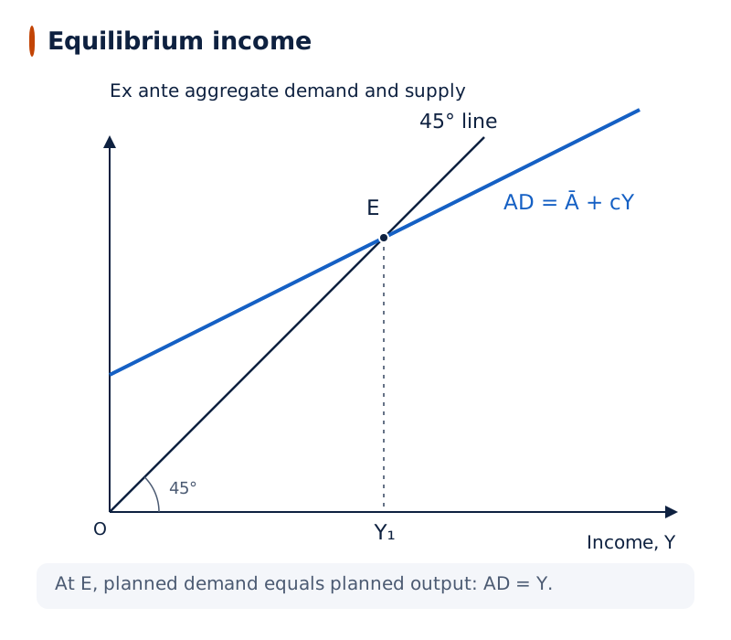
The vertical axis shows ex ante aggregate demand and supply; the horizontal axis shows Y. An upward-sloping demand line crosses the steeper 45° line at E, the equilibrium point. A dotted vertical projects E onto Y₁, the equilibrium income.
Drawn by One Young India. See Fig. 4.6 in your NCERT textbook
How does the algebraic method work?
- Set planned output equal to planned demand: Y = C̄ + Ī + cY.
- Move induced consumption to the left: Y − cY = C̄ + Ī.
- Factor out income: Y(1 − c) = C̄ + Ī.
- Divide by 1 − c to obtain equilibrium income: Y = (C̄ + Ī)/(1 − c).
Y = Ā/(1 − c)
Worked example 3. Given C = 40 + 0.8Y and autonomous investment of 10 units, calculate equilibrium income.
Answer: Total autonomous expenditure is 40 + 10 = 50 units. Equilibrium requires Y = 50 + 0.8Y. Thus 0.2Y = 50 and Y = 250 units. Planned demand at this income is 50 + 0.8 × 250 = 250 units.
The algebra and graph express the same condition. The equation finds the income where the demand function gives expenditure equal to output; the graph locates that equality at the intersection with the 45° line.
Why does the accounting identity not guarantee equilibrium?
The equality between actual output and actual consumption plus investment is an accounting identity, an equality that holds because of how the actual quantities are recorded. It includes investment arising from unintended inventory changes.
Planned demand equals planned supply only at equilibrium. If producers plan more output than buyers plan to purchase, the demand equation does not equal the planned output. The unsold output remains in warehouses as an unintended accumulation of inventories.
How do inventories reconcile the actual values?
- Producers plan output using their expectations of demand.
- Actual sales may fall below the planned level, leaving more goods unsold.
- The additional unsold goods enter actual investment as inventory accumulation.
- Actual output therefore still equals actual consumption plus actual investment, although the original plans were inconsistent.
Note: Unintended stock accumulation is included in ex post investment. Its inclusion preserves the accounting identity; it does not show that the firms intended to hold those extra stocks.
Stock accumulation signals excess supply relative to demand. Producers reduce output to respond to it. Reduced production also reduces factor payments and income, which affects consumption demand. This connection makes inventories part of the explanation of adjustment.
Worked example 4. Total autonomous expenditure is ₹50 crore, MPS is 0.2 and income is ₹4,000 crore. Calculate ex ante aggregate demand and decide whether the economy is in equilibrium.
Answer: MPC = 1 − 0.2 = 0.8. Aggregate demand is ₹50 crore + 0.8 × ₹4,000 crore = ₹3,250 crore. Demand is ₹750 crore below output, so the economy is not in equilibrium. Unsold output produces unintended inventory accumulation.
This example compares planned demand with the stated output. The relevant equality is not automatically satisfied by substituting actual investment after stock changes. The distinction between a planned expenditure function and an accounting record is essential.
How do autonomous changes affect equilibrium income?
A change in autonomous consumption or investment changes total autonomous expenditure. Holding c constant, a rise in Ā shifts the demand line upwards in parallel; a fall shifts it downwards. Equilibrium income changes because the intersection with the 45° line moves.
A parametric shift is a change in a line caused by changing one of the constants determining it. Changing the intercept gives a parallel shift. Changing the slope causes the line to swing rather than move in parallel.
What happens when autonomous investment rises?
Worked example 5. Consumption is C = 40 + 0.8Y. Autonomous investment rises from 10 to 20 units. Calculate the original and new equilibrium incomes.
Answer: Initially, Y = (40 + 10)/(1 − 0.8) = 250 units. After the rise, Y = (40 + 20)/(1 − 0.8) = 300 units. Investment increases by 10 units, while equilibrium income increases by 50 units.
At the original output, the higher investment creates demand exceeding current output. The original equilibrium therefore no longer matches buyers' and suppliers' plans. Production increases, and the additional income generates further consumption expenditure.
What the figure shows
An increase in autonomous expenditure
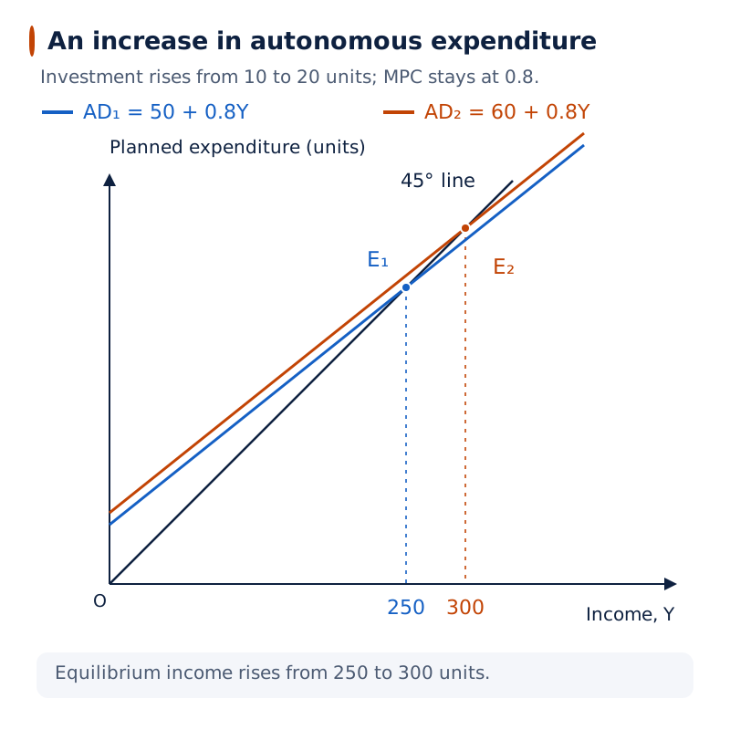
AD₁ and AD₂ denote the initial and higher demand lines. They are parallel. Their intersections with the 45° line are E₁ and E₂, the old and new equilibrium points. The new intersection lies higher and farther right.
Drawn by One Young India. See Fig. 4.7 in your NCERT textbook
A change in consumption demand can also arise from a change in c. That alters the slope of the demand line. It must be distinguished from changing C̄, which alters the intercept without changing the slope.
Autonomous does not mean unexplained by any outside influence. Credit availability and interest rates can affect investment. The point is that investment is treated as independent of the income being determined within this particular model.
How does the investment multiplier mechanism operate?
The investment multiplier is the ratio of the total increase in equilibrium final-goods output to the initial increase in autonomous expenditure. The initial increase becomes income, part of which is spent again, generating further rounds of production and income.
Production employs factors of production: labour, capital, land and entrepreneurship. Their payments include wages, interest, rent and profit. In the absence of indirect taxes or subsidies, the value of output is distributed as these factor incomes.
What happens in successive rounds?
- An autonomous investment increase of 10 units raises demand and induces 10 units of extra output.
- The extra output creates additional factor income of 10 units.
- With MPC of 0.8, the next consumption increase is 0.8 × 10, generating further demand and production.
- Income from that production generates another consumption increase of 0.8² × 10. The process continues through progressively smaller rounds.
| Round | Consumption increment | Demand increment | Output or income increment |
|---|---|---|---|
| 1 | 0 | 10, autonomous increase | 10 |
| 2 | 0.8 × 10 | 0.8 × 10 | 0.8 × 10 |
| 3 | 0.8² × 10 | 0.8² × 10 | 0.8² × 10 |
| 4 | 0.8³ × 10 | 0.8³ × 10 | 0.8³ × 10 |
The output increments form a geometric series, with each successive term obtained by multiplying the previous term by 0.8. Adding all the rounds gives 10/(1 − 0.8) = 50 units, the total increase in equilibrium income.
Here ΔĀ denotes the initial autonomous expenditure increase and ΔY the total equilibrium income increase. When the autonomous change is in investment, ΔĀ equals ΔI, the investment increase.
ΔY/ΔĀ = 1/(1 − c)
Since s = 1 − c, the multiplier also equals 1/s. As c becomes larger, the multiplier increases: more of each additional income is spent on consumption, generating a larger total output response through subsequent rounds.
Note: The multiplier describes the total change after the successive rounds. The initial investment increase of 10 units and the eventual income increase of 50 units are different stages of the same adjustment.
What is the paradox of thrift?
The paradox of thrift states that when everyone increases the proportion of income saved, total saving will not increase: it will either decline or remain unchanged. People becoming more thrifty can end up saving less or the same as before.
The reason is that spending decisions also affect total income. A higher saving propensity means a lower consumption propensity. At the initial income, lower consumption reduces demand, leaving excess supply. Output and income then contract through successive rounds.
How does the numerical example show the paradox?
Initially, autonomous consumption is 40 units, investment is 10 units and MPC is 0.8. Equilibrium income is 250 units. Suppose MPC falls to 0.5 because of a change in expenditure behaviour originating outside the model.
At the original income, demand falls by (0.8 − 0.5) × 250 = 75 units. Producers cut output in response to unsold stocks. Falling factor payments reduce income, and further consumption decreases follow at the new MPC of 0.5.
Worked example 6. With autonomous consumption of 40 units and investment of 10 units, compare equilibrium income and saving when MPC falls from 0.8 to 0.5.
Answer: Initial income is 50/(1 − 0.8) = 250 units; saving is 250 − (40 + 0.8 × 250) = 10 units. New income is 50/(1 − 0.5) = 100 units; saving is 100 − (40 + 0.5 × 100) = 10 units.
The total output reduction is 75/(1 − 0.5) = 150 units. Although the proportion saved rises, the income to which it applies falls. Aggregate saving therefore remains unchanged in this example.
What the figure shows
Downward swing of aggregate demand
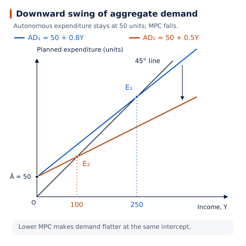
The initial and new demand lines share the intercept Ā. The new line is flatter. Its intersection E₂ with the 45° line lies below and left of the original equilibrium E₁, showing lower equilibrium income and demand.
Drawn by One Young India. See Fig. 4.8 in your NCERT textbook
The unchanged intercept is crucial: the example changes the propensity to consume while keeping autonomous expenditure at 50 units. This is a downward swing caused by a lower slope, rather than a parallel downward shift.
How are equilibrium, employment and demand imbalances connected?
Full employment income is the income level at which all factors of production are fully employed in production. Given the quantities of other factors, equilibrium output also determines employment. However, equilibrium by itself does not mean that everyone is employed.
The condition Y = AD shows that planned demand and output match. It means income will not change if the economy is left to itself, even when unemployment exists. It does not establish that all available resources are being used.
What are deficient demand and excess demand?
Deficient demand is the situation where demand is insufficient to employ all factors of production and equilibrium output is below full-employment output. It leads to a decline in prices in the long run.
Excess demand arises when demand exceeds the output produced at full employment. The equilibrium output implied by demand is above the full-employment level. This situation leads to a rise in prices in the long run.
| Situation | Demand relative to full-employment output | Long-run price effect |
|---|---|---|
| Deficient demand | Insufficient to employ all factors | Prices decline |
| Excess demand | Exceeds output at full employment | Prices rise |
How does introducing government affect demand?
Government expenditure, denoted by G, adds to demand for final goods and services. Taxes, denoted by T, take income away from households. Both are treated as autonomous in this extension.
Disposable income, denoted by Yd, is household income after taxes: Yd = Y − T. Consumption depends on this disposable income, so the equilibrium equation becomes Y = C̄ + Ī + G + c(Y − T).
The term G − cT adds to autonomous expenditure. Thus spending and taxes enter differently: government purchases add directly to demand, while taxes affect the income available for consumption. The two-sector analysis sets this government extension aside to focus on consumption and investment.
Note: Keep the time qualification: deficient demand and excess demand have the stated price effects in the long run. The short-run income model begins with a fixed price level.
Glossary
- Ex ante — Planned values of consumption, investment or output before the outcome of the period is known.
- Ex post — Actual values realised and recorded after economic activities have taken place during a period.
- Autonomous consumption — Consumption independent of income, including consumption that occurs when income is zero.
- Induced consumption — The part of consumption that depends on income and changes as income changes.
- Marginal propensity to consume — The change in consumption expenditure per unit change in income.
- Marginal propensity to save — The change in saving per unit change in income, equal to one minus MPC.
- Average propensity to consume — Total consumption expenditure per unit of income, calculated by dividing consumption by income.
- Average propensity to save — Total saving per unit of income, calculated by dividing saving by income.
- Autonomous investment — Given investment expenditure that is treated as independent of income in the model.
- Inventory investment — A change in stocks of unsold output held by a producer during a period.
- Aggregate demand — Planned total expenditure on final goods and services, including consumption and investment in the two-sector model.
- Effective demand principle — Aggregate output is determined solely by aggregate demand under the model's fixed-price supply assumptions.
- Investment multiplier — The ratio of total equilibrium output increase to the initial increase in autonomous expenditure.
- Paradox of thrift — A rise in the saving propensity of everyone leaves aggregate saving unchanged or lower.
- Full employment income — The income level at which all factors of production are fully employed in production.
Common errors and misconceptions
- Misconception: Ex ante and ex post are interchangeable. Correct: Ex ante describes plans; ex post describes actual outcomes, which can differ because sales and inventories change unexpectedly.
- Misconception: MPC uses total consumption divided by total income. Correct: That ratio is APC. MPC uses the change in consumption divided by the change in income.
- Misconception: Autonomous investment cannot change. Correct: It is independent of income in this model, but credit availability and interest rates can affect investment.
- Misconception: Actual output equalling actual consumption plus investment proves equilibrium. Correct: Actual investment includes unintended stock changes. Equilibrium requires equality of the planned quantities.
- Misconception: A rise in investment and a rise in MPC move the demand line identically. Correct: Higher autonomous investment shifts it upwards in parallel; higher MPC changes its slope.
- Misconception: A greater saving propensity necessarily raises total saving. Correct: Lower demand can reduce income, leaving aggregate saving unchanged or lower through the paradox of thrift.
- Misconception: Equilibrium guarantees full employment. Correct: Planned demand can match output while resources remain unemployed; equilibrium and full employment are different conditions.
- Misconception: Deficient demand changes prices immediately within the fixed-price model. Correct: The stated decline in prices concerns the long run, while the short-run analysis holds prices fixed.
Exam-style questions with model answers
Q1. Distinguish between ex ante investment and ex post investment. [2 marks]
- Ex ante investment is the investment planned by producers for a period, including planned additions to their stocks.
- Ex post investment is the investment actually realised, including inventory changes caused by sales differing from their expected level.
Q2. A producer plans an inventory addition of ₹100, but unexpectedly sells ₹30 worth of goods from that stock. Find planned and actual investment. [2 marks]
- Planned, or ex ante, investment is ₹100, the intended addition to the producer's stock.
- Actual, or ex post, investment is ₹100 − ₹30 = ₹70, because unexpected sales reduce the inventory addition.
Q3. Define marginal propensity to consume and marginal propensity to save, and derive their relationship. [3 marks]
- Marginal propensity to consume, c, is the change in consumption per unit change in income: c = ΔC/ΔY. Here Δ means change, C consumption and Y income.
- Marginal propensity to save, s, is the change in saving per unit change in income: s = ΔS/ΔY, where S denotes saving.
- Since S = Y − C, dividing ΔS = ΔY − ΔC by ΔY gives s = 1 − c. Thus MPC + MPS = 1.
Q4. In a fixed-price two-sector economy, total autonomous expenditure is ₹50 crore, marginal propensity to save is 0.2 and output or income is ₹4,000 crore. Calculate planned demand and explain whether this is equilibrium. [4 marks]
- Marginal propensity to consume equals one minus marginal propensity to save, so c = 1 − 0.2 = 0.8.
- Planned aggregate demand equals autonomous expenditure plus induced consumption: ₹50 crore + 0.8 × ₹4,000 crore = ₹3,250 crore.
- Output is ₹4,000 crore, so planned demand is lower than output by ₹4,000 crore − ₹3,250 crore = ₹750 crore.
- This is not equilibrium because planned demand and output differ. The unsold output appears as unintended inventory accumulation, giving producers a reason to reduce production.
Q5. In a two-sector economy with fixed prices and interest rate and unused resources, consumption is C = 40 + 0.8Y, where C is consumption and Y is income, in units. Autonomous investment rises from 10 to 20 units. Calculate both equilibrium incomes and explain the multiplier mechanism. [6 marks]
- Initially, autonomous expenditure is autonomous consumption plus investment, or 40 + 10 = 50 units. The marginal propensity to consume is 0.8.
- Equilibrium requires planned output to equal planned demand: Y = 50 + 0.8Y. Therefore initial equilibrium income is 50/(1 − 0.8) = 250 units.
- After investment rises, autonomous expenditure becomes 40 + 20 = 60 units. New equilibrium income is 60/(1 − 0.8) = 300 units.
- The investment increase of 10 units initially raises production and factor income by 10 units as firms respond to additional demand.
- Recipients consume 0.8 of additional income. The next demand and output increase is 0.8 × 10, followed by 0.8² × 10 and further rounds.
- The multiplier, the total income increase divided by the initial investment increase, is 1/(1 − 0.8) = 5. Income consequently rises by 50 units, from 250 to 300.
Q6. In a fixed-price two-sector economy, autonomous consumption is 40 units and autonomous investment is 10 units. Marginal propensity to consume falls from 0.8 to 0.5. Calculate income and saving before and after the change, and explain the paradox of thrift. [5 marks]
- Autonomous expenditure remains 40 + 10 = 50 units. Initial equilibrium income is 50/(1 − 0.8) = 250 units.
- Initial saving equals income minus consumption: 250 − (40 + 0.8 × 250) = 10 units.
- With marginal propensity to consume reduced to 0.5, new equilibrium income is 50/(1 − 0.5) = 100 units.
- New saving is 100 − (40 + 0.5 × 100) = 10 units. Thus aggregate saving remains unchanged even though the saving propensity has increased.
- Lower consumption demand reduces output and income. The paradox of thrift means that everyone trying to save a greater proportion of income can leave total saving unchanged or lower; this example shows the unchanged outcome.
Q7. Explain why equilibrium need not imply full employment, and distinguish deficient demand from excess demand, including their long-run price effects. [4 marks]
- Equilibrium means planned aggregate demand equals planned output. Income can remain at that level even when unemployment exists, so this equality does not guarantee full employment.
- Full employment income is the level at which all factors of production are fully employed in the production process.
- Deficient demand means demand is insufficient to employ all factors, placing equilibrium output below full-employment output. It leads to declining prices in the long run.
- Excess demand means demand exceeds output at full employment. It leads to rising prices in the long run.
Q8. Explain how a change in the intercept differs from a change in the slope of the aggregate demand line. [3 marks]
- The aggregate demand function is AD = Ā + cY, where AD is planned demand, Ā autonomous expenditure, c marginal propensity to consume and Y income.
- Changing Ā changes the vertical intercept. With c unchanged, an increase shifts the line upwards in parallel and a decrease shifts it downwards in parallel.
- Changing c changes the slope. A lower marginal propensity to consume makes the line flatter and swings it downwards while the autonomous expenditure intercept remains unchanged.
Key takeaways
- Ex ante quantities describe plans; ex post quantities describe actual outcomes, including unintended changes in inventories.
- Consumption combines an autonomous component with induced spending that changes with income according to the marginal propensity to consume.
- Marginal propensities use changes in income, consumption and saving; average propensities use their total values.
- Equilibrium requires planned demand to equal planned output, whereas the accounting identity includes actual inventory investment.
- An increase in autonomous expenditure shifts aggregate demand upwards and raises equilibrium income through successive spending rounds.
- The multiplier becomes larger as the marginal propensity to consume rises, increasing the total response to autonomous spending.
- The paradox of thrift links greater intended saving with falling income, leaving aggregate saving unchanged or lower.
- Equilibrium need not ensure full employment; deficient demand and excess demand have different long-run effects on prices.
Test yourself
What does ceteris paribus mean?
It means other things remaining equal: other variables are held constant while a particular relationship is investigated.
Why can consumption occur at zero income?
Autonomous consumption is independent of income and remains present even when the income-dependent component is zero.
If MPC is 0.8, what is MPS?
MPS is 1 − 0.8 = 0.2, because the marginal propensities to consume and save add to one.
Why is the autonomous investment line horizontal?
Investment is assumed independent of income, so its planned amount stays unchanged as the income level varies.
What does the 45° line show in the equilibrium diagram?
Every point has equal horizontal and vertical coordinates, allowing planned expenditure to be compared with the same value of output.
What distinguishes a parallel demand shift from a downward swing?
A parallel shift changes autonomous expenditure while keeping the slope unchanged. A downward swing occurs when marginal propensity to consume falls.
Why can actual investment exceed planned investment?
Unexpectedly low sales can create unintended inventory accumulation, which becomes part of actual investment even though it was not planned.
Why can equilibrium coexist with unemployment?
Planned demand may equal output below full employment. Equality of these plans does not ensure that all factors are employed.
Write about it
Turn a question from this chapter into a paper.
The Writing Studio has a structure guide, a rubric and citation tools for 15 formats, from essays to research papers. Drafting is free with an account. Learnacy Essential adds feedback from an AI writing coach and submission to The OYI Review.
Learnacy Essential is ₹1,499 for the year. Publication depends on review and is not guaranteed.