Electric Charges and Fields | CBSE Class 12 Physics Notes

This note covers electric charge, conductors and insulators, conservation and quantisation, Coulomb’s law, superposition, electric fields and field lines, electric flux, dipoles, continuous charge distributions, Gauss’s law, and fields due to a charged wire, plane sheet and spherical shell.

What is electric charge, and how do materials become charged?

Positive and negative charge

Electric charge has two kinds, positive and negative. Like charges repel, while unlike charges attract. A glass rod rubbed with silk becomes positively charged; the silk becomes negatively charged. A plastic rod rubbed with fur becomes negatively charged.

A neutral material already contains charged constituents. Its positive and negative charges balance. Charging changes this balance: a body that loses electrons becomes positively charged, while one that gains electrons becomes negatively charged. Rubbing transfers electrons rather than creating new charge.

Definition: Electrostatics is the study of forces, fields and potentials associated with static electric charges.

The SI unit of electric charge is the coulomb, written as $\mathrm{C}$. One coulomb is the charge passing through a wire in $1\,\mathrm{s}$ when the current is $1\,\mathrm{A}$: $1\,\mathrm{C}=1\,\mathrm{A\,s}$. Smaller units include $1\,\mu\mathrm{C}=10^{-6}\,\mathrm{C}$ and $1\,\mathrm{mC}=10^{-3}\,\mathrm{C}$.

How do conductors differ from insulators?

A metal spoon held in the hand loses charge through the body to earth. A metal rod held by a wooden or plastic handle can show charging because the handle interrupts that conducting route. The distinction concerns charge mobility, not the presence or absence of charged particles.

A gold-leaf electroscope detects charge. When a charged object touches its metal knob, charge reaches two thin gold leaves attached to the rod. The leaves diverge, and the extent of divergence indicates the amount of charge.

What are the three basic properties of electric charge?

Additivity, conservation and quantisation

Additivity means that total charge is the algebraic sum of individual charges. Charge is a scalar, so signs must be retained, but no directions are added. For a collection of charges, the total charge is $$Q=q_1+q_2+\cdots+q_n.$$

Conservation of charge means that the net charge of an isolated system remains unchanged. Charge may move between bodies within the system. The charge gained by one body is balanced by the charge lost by another, as when glass and silk are rubbed together.

Quantisation means that free charge occurs in integral multiples of the elementary charge. The quantisation relation is $$q=ne,\qquad n=0,\pm1,\pm2,\ldots$$ Here $e\approx1.6\times10^{-19}\,\mathrm{C}$, and $n$ is an integer. The electron carries $-e$; the proton carries $+e$.

Macroscopic charges involve enormous numbers of elementary charges. Their discrete steps are then too small to matter in many calculations, so a continuous description is useful. At microscopic scales involving a few electrons, the discrete nature cannot be ignored.

Note: Conservation concerns the total charge of an isolated system. It does not require each individual body to retain its original charge.

Worked example 1. Electrons leave one body and enter another at $10^9$ electrons per second. Find the time needed to transfer a charge of magnitude $1\,\mathrm{C}$.

Formula: $I=\dot{N}e$, followed by $t=Q/I$, where $I$ is the magnitude of the rate of charge transfer.

Answer: Calculate the charge transferred in $\text{1 s}$, then divide the required charge by that rate.

1. Substitute the electron rate: $$I=(10^9\,\mathrm{s}^{-1})(1.6\times10^{-19}\,\mathrm{C})=1.6\times10^{-10}\,\mathrm{C\,s}^{-1}.$$
2. Calculate the time: $$t=\frac{1\,\mathrm{C}}{1.6\times10^{-10}\,\mathrm{C\,s}^{-1}}=6.25\times10^9\,\mathrm{s}.$$
3. Using a year of $365$ days, convert the result: $$t=\frac{6.25\times10^9\,\mathrm{s}}{365\times24\times3600\,\mathrm{s\,year}^{-1}}\approx198.2\,\mathrm{years}.$$ This is approximately $200$ years. The receiving body becomes negatively charged.

How does Coulomb’s law describe the force between charges?

Coulomb’s law gives the electrostatic force between stationary point charges. A charged body can be treated as a point charge when its dimensions are much smaller than its separation from the other body. The force acts along the line joining the charges.

For charges $q_1$ and $q_2$ separated by $r$ in vacuum, the force magnitude is $$F=k\frac{|q_1q_2|}{r^2},\qquad k=\frac{1}{4\pi\varepsilon_0}.$$ Here $F$ is in newtons, charges are in coulombs and separation is in metres.

The permittivity of free space is $\varepsilon_0=8.854\times10^{-12}\,\mathrm{C^2\,N^{-1}\,m^{-2}}$, giving $k\approx9\times10^9\,\mathrm{N\,m^2\,C^{-2}}$. For a fixed pair of charges, the force follows an inverse-square dependence on separation.

How are direction and signs included?

Let $\hat{\mathbf r}_{21}$ point from the first charge towards the second, and let $\mathbf F_{21}$ be the force on the second charge due to the first. The vector form is $$\mathbf F_{21}=\frac{q_1q_2}{4\pi\varepsilon_0r_{21}^2}\hat{\mathbf r}_{21}.$$ The signed product produces repulsion for like charges and attraction for unlike charges.

The two interaction forces satisfy $\mathbf F_{12}=-\mathbf F_{21}$, consistent with Newton’s third law. They act on different bodies. The vacuum form should not be applied indiscriminately to charges embedded in matter, whose charged constituents also affect the interaction.

Worked example 2. Two small spheres carry $2\times10^{-7}\,\mathrm{C}$ and $3\times10^{-7}\,\mathrm{C}$, separated by $30\,\mathrm{cm}$ in air. Calculate their mutual force using $k\approx9\times10^9\,\mathrm{N\,m^2\,C^{-2}}$.

Formula: $F=k|q_1q_2|/r^2$.

Answer: Both charges are positive, so the force is repulsive.

1. Convert the separation: $$r=30\,\mathrm{cm}=\text{0.30 m}.$$
2. Substitute in Coulomb’s law: $$F=\frac{(9\times10^9\,\mathrm{N\,m^2\,C^{-2}})(2\times10^{-7}\,\mathrm{C})(3\times10^{-7}\,\mathrm{C})}{(0.30\,\mathrm{m})^2}.$$
3. Evaluate: $$F=\frac{5.4\times10^{-4}\,\mathrm{N\,m^2}}{0.09\,\mathrm{m^2}}=6.0\times10^{-3}\,\mathrm{N}.$$ Each sphere experiences this magnitude, directed away from the other sphere.

How do superposition and electric field simplify many-charge problems?

The superposition principle states that the force due to each source charge is unaffected by other charges. The resultant force is the vector sum of those individual forces. Adding their magnitudes alone is valid only when the relevant directions justify it.

An electric field describes the electrical environment created by source charges. Operationally, it is force per unit positive test charge, with the test charge small enough not to disturb the sources: $$\mathbf E=\lim_{q_0\to0}\frac{\mathbf F}{q_0}.$$

The SI unit of electric field is $\mathrm{N\,C^{-1}}$. The field exists independently of the chosen test charge. Once it is known, the force on a charge is $\mathbf F=q\mathbf E$. A negative charge experiences force opposite to the field.

The field of a point charge is $$\mathbf E=\frac{Q}{4\pi\varepsilon_0r^2}\hat{\mathbf r}.$$ The unit vector points from the source to the observation point. A positive source gives an outward field; a negative source gives an inward field. Equal distances from a single point charge have equal field magnitudes.

Adding fields before finding force

For several sources, $\mathbf E=\mathbf E_1+\mathbf E_2+\cdots+\mathbf E_n$. Determine each direction and resolve components before summing. A symmetrical arrangement may make the resultant vanish even though individual fields are non-zero. Three equal charges at an equilateral triangle’s vertices give zero resultant at its centroid.

Worked example 3. An electron starts from rest and falls $1.5\,\mathrm{cm}$ in an upward field of magnitude $2.0\times10^4\,\mathrm{N\,C^{-1}}$. Find its fall time, then the proton’s fall time when the field is reversed.

Formula: $F=eE$, $a=F/m$, and $t=\sqrt{2h/a}$. Use $m_e=9.11\times10^{-31}\,\mathrm{kg}$ and $m_p=1.67\times10^{-27}\,\mathrm{kg}$.

Answer: Use $h=\text{0.015 m}$. In each case the electric force is downward.

1. The common force magnitude is $$F=(1.6\times10^{-19}\,\mathrm{C})(2.0\times10^4\,\mathrm{N\,C^{-1}})=3.2\times10^{-15}\,\mathrm{N}.$$
2. The electron’s acceleration is $$a_e=\frac{3.2\times10^{-15}\,\mathrm{N}}{9.11\times10^{-31}\,\mathrm{kg}}\approx3.51\times10^{15}\,\mathrm{m\,s^{-2}}.$$
3. Its time is $$t_e=\sqrt{\frac{2(0.015\,\mathrm{m})}{3.51\times10^{15}\,\mathrm{m\,s^{-2}}}}\approx2.92\times10^{-9}\,\mathrm{s}.$$
4. The proton’s acceleration is $$a_p=\frac{3.2\times10^{-15}\,\mathrm{N}}{1.67\times10^{-27}\,\mathrm{kg}}\approx1.92\times10^{12}\,\mathrm{m\,s^{-2}}.$$
5. Its time is $$t_p=\sqrt{\frac{2(0.015\,\mathrm{m})}{1.92\times10^{12}\,\mathrm{m\,s^{-2}}}}\approx1.25\times10^{-7}\,\mathrm{s}.$$ Both accelerations greatly exceed $9.8\,\mathrm{m\,s^{-2}}$, justifying neglect of gravity.

The heavier proton takes longer. Electric acceleration depends on charge and mass, whereas the time for free fall under gravity, with the same initial conditions, is independent of the falling body’s mass.

How do electric field lines represent direction and strength?

An electric field line is a curve whose tangent gives the direction of the net electric field. Its arrow specifies which way along that tangent the field points. Although sketches are usually drawn on paper, field lines represent curves in three-dimensional space.

Relative line density indicates relative field strength. Crowded lines represent stronger fields; widely separated lines represent weaker fields. Density is considered per unit area perpendicular to the lines. The total number drawn is a choice, not a directly measurable count of physical threads.

• Lines begin at positive charges and end at negative charges; for an isolated charge, they can begin or end at infinity.
• In a charge-free region, the lines are continuous curves without breaks.
• Two field lines cannot cross, because a crossing would assign two field directions at the same point.
• Electrostatic field lines do not form closed loops.

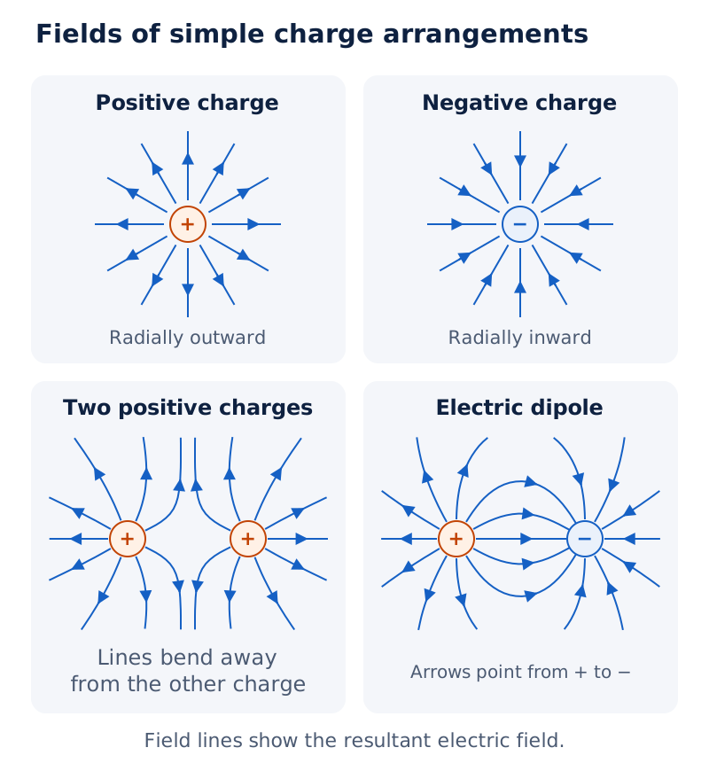
Four panels show outward radial arrows around a positive charge, inward arrows around a negative charge, curved lines around two positive charges, and lines directed from the positive to the negative member of a dipole.

See Fig. 1.14 in your NCERT textbook

A field-line sketch must describe the resultant field. It is not made by drawing separate, intersecting sets of lines for each charge. Superposition is performed on field vectors first; the final pattern represents their combined direction at every point.

Worked example 4. Charges $+10^{-8}\,\mathrm{C}$ and $-10^{-8}\,\mathrm{C}$ lie $0.10\,\mathrm{m}$ apart, with the positive charge on the left. Find the field at their midpoint, at a point $0.05\,\mathrm{m}$ left of the positive charge, and at the upper equilateral-triangle vertex.

Formula: $E=k|q|/r^2$, followed by vector addition.

Answer: Use the directions away from the positive charge and towards the negative charge.

1. At the midpoint, each distance is $\text{0.05 m}$. Each field has magnitude $$E_1=E_2=\frac{(9\times10^9\,\mathrm{N\,m^2\,C^{-2}})(10^{-8}\,\mathrm{C})}{(0.05\,\mathrm{m})^2}=3.6\times10^4\,\mathrm{N\,C^{-1}}.$$ Both point right, so $$E_A=3.6\times10^4\,\mathrm{N\,C^{-1}}+3.6\times10^4\,\mathrm{N\,C^{-1}}=7.2\times10^4\,\mathrm{N\,C^{-1}}.$$
2. At the left-hand point, the nearer field is leftward. The farther field is rightward and equals $$E_2=\frac{(9\times10^9\,\mathrm{N\,m^2\,C^{-2}})(10^{-8}\,\mathrm{C})}{(0.15\,\mathrm{m})^2}=4.0\times10^3\,\mathrm{N\,C^{-1}}.$$ The resultant is leftward: $$E_B=3.6\times10^4\,\mathrm{N\,C^{-1}}-4.0\times10^3\,\mathrm{N\,C^{-1}}=3.2\times10^4\,\mathrm{N\,C^{-1}}.$$
3. At the upper vertex, both distances are $\text{0.10 m}$, giving $$E_1=E_2=\frac{(9\times10^9\,\mathrm{N\,m^2\,C^{-2}})(10^{-8}\,\mathrm{C})}{(0.10\,\mathrm{m})^2}=9.0\times10^3\,\mathrm{N\,C^{-1}}.$$ Vertical components cancel, while horizontal components add: $$E_C=2(9.0\times10^3\,\mathrm{N\,C^{-1}})\cos60^\circ=9.0\times10^3\,\mathrm{N\,C^{-1}},$$ directed rightward.

What are electric flux and continuous charge density?

Flux measures the field through a surface

Electric flux depends on the field, the area and the surface’s orientation. For a small planar element, the flux relation is $$\Delta\Phi=\mathbf E\cdot\Delta\mathbf S=E\Delta S\cos\theta.$$ The angle is measured between the field and the area’s normal, not between the field and the plane.

The SI unit of electric flux is $\mathrm{N\,m^2\,C^{-1}}$. For a closed surface, the area vector points outward. Outward field components give positive flux and inward components negative flux. A field tangent to the surface contributes no flux through it.

For a uniform field over a flat surface, $\Phi=ES\cos\theta$. For a curved surface or varying field, divide the surface into small elements and add their fluxes. In the limit, the surface-integral form is $$\Phi=\int_S\mathbf E\cdot\mathrm d\mathbf S.$$

Flux is analogous to flow through an area, but electric flux does not mean that a material substance is flowing through the surface. Field lines provide a useful visual interpretation through their relative density and orientation.

How are extended charge distributions described?

A continuous charge distribution averages over microscopic charges. Each chosen element is small on the scale of the object but contains many charged constituents. This description does not overturn quantisation; it makes the microscopic granularity unnecessary for the calculation.

The SI unit of linear charge density is $\mathrm{C\,m^{-1}}$. The SI unit of surface charge density is $\mathrm{C\,m^{-2}}$, and the SI unit of volume charge density is $\mathrm{C\,m^{-3}}$. Charge density may vary with position.

For a volume element, the field contribution is $\Delta\mathbf E=k\rho\Delta V\hat{\mathbf r}'/r'^2$. Here $r'$ is the distance from that element to the observation point. Summing the contributions applies the same superposition principle used for discrete charges.

How are the axial and equatorial fields of an electric dipole derived?

An electric dipole consists of equal and opposite point charges separated by a distance. Write their magnitudes as $q$ and their separation as $2a$. The dipole moment points from the negative charge towards the positive charge: $$\mathbf p=q(2a)\hat{\mathbf p}.$$

The SI unit of dipole moment is $\mathrm{C\,m}$. Zero net charge does not imply zero field, because the two charges occupy different positions. Their fields must be added as vectors at the observation point.

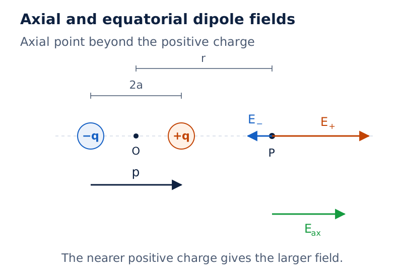
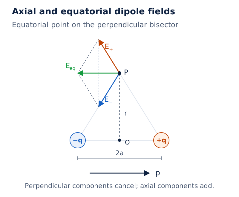
The axial panel places the observation point beyond the positive charge and shows opposing field arrows. The equatorial panel marks the midpoint distance and shows the component construction. The dipole moment arrow points from the negative charge towards the positive charge.

See Fig. 1.17 in your NCERT textbook

Derivation: Field on the axis

Choose a point at distance $r$ from the midpoint, beyond the positive charge, with $r>a$. The unit vector $\hat{\mathbf p}$ follows the dipole moment.

1. The distances from the positive and negative charges are $r-a$ and $r+a$. Their fields are $$\mathbf E_+=\frac{kq}{(r-a)^2}\hat{\mathbf p},\qquad\mathbf E_-=-\frac{kq}{(r+a)^2}\hat{\mathbf p}.$$
2. Add the opposite contributions: $$\mathbf E_{\mathrm{ax}}=kq\left[\frac{1}{(r-a)^2}-\frac{1}{(r+a)^2}\right]\hat{\mathbf p}.$$
3. Combine the fractions and use $p=2qa$: $$\mathbf E_{\mathrm{ax}}=\frac{4kqar}{(r^2-a^2)^2}\hat{\mathbf p}=\frac{2kpr}{(r^2-a^2)^2}\hat{\mathbf p}.$$
4. For $r\gg a$, neglect $a^2$ against $r^2$: $$\mathbf E_{\mathrm{ax}}\approx\frac{2k\mathbf p}{r^3}.$$

Axial result: At an exterior axial point, the resultant field is along the dipole moment. The inverse-cube expression is a distant-point approximation for a finite dipole.

Derivation: Field in the equatorial plane

Choose a point at distance $r$ from the centre in the perpendicular bisector plane.

1. Both charges are at distance $\sqrt{r^2+a^2}$, so $$E_+=E_-=\frac{kq}{r^2+a^2}.$$
2. The components perpendicular to the dipole axis cancel. The axial components add opposite to $\hat{\mathbf p}$, with projection factor $a/\sqrt{r^2+a^2}$.
3. Therefore, $$\mathbf E_{\mathrm{eq}}=-2\frac{kq}{r^2+a^2}\frac{a}{\sqrt{r^2+a^2}}\hat{\mathbf p}=-\frac{k\mathbf p}{(r^2+a^2)^{3/2}}.$$
4. For $r\gg a$, $$\mathbf E_{\mathrm{eq}}\approx-\frac{k\mathbf p}{r^3}.$$

Equatorial result: The field is opposite to the dipole moment. At equal large distances, the axial magnitude is twice the equatorial magnitude. Both decrease as $r^{-3}$, faster than the $r^{-2}$ field of an isolated point charge.

A point dipole is the ideal limit in which separation tends to zero while dipole moment remains finite. The distant-point expressions become exact for this idealisation at non-zero distances from it.

What happens to a dipole in an external electric field?

In a uniform external field, the two charges experience equal and opposite forces. Their resultant force is zero, but their different points of application can produce a torque. Thus zero net force does not imply an absence of rotational effect.

Derivation: Torque on a dipole

Let $\theta$ be the angle between the dipole moment and the uniform field.

1. The two forces are $$\mathbf F_+=q\mathbf E,\qquad\mathbf F_-=-q\mathbf E,\qquad\mathbf F_{\mathrm{net}}=\mathbf0.$$
2. The perpendicular separation of their lines of action is $$d=2a\sin\theta.$$
3. The couple has torque magnitude $$\tau=(qE)(2a\sin\theta)=pE\sin\theta.$$
4. The vector direction follows the cross product: $$\boldsymbol\tau=\mathbf p\times\mathbf E.$$

Torque result: The torque tends to align the dipole with the field. It vanishes when the dipole is parallel or antiparallel to the field. The torque unit is $\mathrm{N\,m}$.

Polar molecules and non-uniform fields

In polar molecules, the centres of positive and negative charge do not coincide, producing a permanent dipole moment. Water is an example. In CO₂ and CH₄ these centres coincide, so there is no permanent dipole moment, although an applied field can induce one.

A non-uniform field can produce a net force as well as a torque. For a dipole parallel to the field, the force is towards increasing field strength; for an antiparallel dipole, it is towards decreasing field strength.

A comb rubbed through dry hair attracts neutral paper because it polarises the paper. The comb’s field is non-uniform, so the induced dipole experiences a net attractive force. Neutrality of the paper therefore does not prevent electrical attraction.

What does Gauss’s law say about a closed surface?

Gauss’s law connects net outward electric flux through a closed surface with the algebraic charge enclosed: $$\oint_S\mathbf E\cdot\mathrm d\mathbf S=\frac{Q_{\mathrm{enc}}}{\varepsilon_0}.$$ The law is valid for any closed surface, regardless of its shape or size.

The field on the left is due to all source charges, including those outside the surface. The right-hand side counts only enclosed charge. An external charge can alter the field at individual surface points without contributing to the net flux through the closed surface.

A Gaussian surface is an imaginary closed surface chosen for applying the law. Avoid passing it through a discrete point charge, where that charge’s field is undefined. It may pass through a continuous charge distribution.

For a centred point charge and spherical surface, the field is normal and has constant magnitude. Multiplying the inverse-square field by the sphere’s area gives flux independent of radius. This illustrates the connection between Gauss’s law and Coulomb’s inverse-square law.

Note: Zero net flux means zero net enclosed charge. It does not establish that there are no charges inside, or that the electric field is zero everywhere on the surface.

Worked calculations using flux

Worked example 5. A cube of side $a=0.1\,\mathrm{m}$ extends from $x=a$ to $x=2a$. The field is $E_x=\alpha\sqrt{x}$, with $E_y=E_z=0$ and $\alpha=800\,\mathrm{N\,C^{-1}\,m^{-1/2}}$. Find its net flux and enclosed charge.

Formula: $\Phi=a^2(E_R-E_L)$, then $Q=\varepsilon_0\Phi$.

Answer: Four faces have zero flux because the field is tangent to them. The left face contributes negatively and the right face positively.

1. The faces lie at $x_L=\text{0.1 m}$ and $x_R=\text{0.2 m}$. Their fields are $$E_L=(800\,\mathrm{N\,C^{-1}\,m^{-1/2}})\sqrt{0.1\,\mathrm{m}}\approx252.982\,\mathrm{N\,C^{-1}},$$ $$E_R=(800\,\mathrm{N\,C^{-1}\,m^{-1/2}})\sqrt{0.2\,\mathrm{m}}\approx357.771\,\mathrm{N\,C^{-1}}.$$
2. Subtract before rounding the final answer: $$\Phi=(0.1\,\mathrm{m})^2(357.771-252.982)\,\mathrm{N\,C^{-1}}\approx1.04789\,\mathrm{N\,m^2\,C^{-1}}.$$
3. Apply Gauss’s law: $$Q=(8.854\times10^{-12}\,\mathrm{C^2\,N^{-1}\,m^{-2}})(1.04789\,\mathrm{N\,m^2\,C^{-1}})\approx9.28\times10^{-12}\,\mathrm{C}.$$

Worked example 6. A cylinder of length $20\,\mathrm{cm}$ and radius $5\,\mathrm{cm}$ is centred at the origin with its axis along the horizontal coordinate axis. The field has magnitude $200\,\mathrm{N\,C^{-1}}$, pointing right on the positive side and left on the negative side. Find the flux and enclosed charge.

Formula: $\Phi=2E\pi R^2$, followed by $Q=\varepsilon_0\Phi$.

Answer: On both ends the field is outward. On the curved side it is tangent, so that side contributes zero flux.

1. Use $R=\text{0.05 m}$. The area of each end is $$A=\pi(0.05\,\mathrm{m})^2\approx7.85398\times10^{-3}\,\mathrm{m^2}.$$
2. Each end contributes $$\Phi_{\mathrm{end}}=(200\,\mathrm{N\,C^{-1}})\pi(0.05\,\mathrm{m})^2\approx1.57080\,\mathrm{N\,m^2\,C^{-1}}.$$
3. The total is $$\Phi=2(1.57080\,\mathrm{N\,m^2\,C^{-1}})+0\,\mathrm{N\,m^2\,C^{-1}}\approx3.14159\,\mathrm{N\,m^2\,C^{-1}}.$$
4. The enclosed charge is $$Q=(8.854\times10^{-12}\,\mathrm{C^2\,N^{-1}\,m^{-2}})(3.14159\,\mathrm{N\,m^2\,C^{-1}})\approx2.78\times10^{-11}\,\mathrm{C}.$$

Gauss’s law determines the net charge in both examples without locating individual charges. Finding the local field from enclosed charge alone is a different task: it requires enough symmetry to simplify the flux integral.

How does Gauss’s law give the field of an infinitely long charged wire?

Consider an infinitely long, thin, straight wire carrying uniform linear charge density $\lambda$. Rotational symmetry makes all points at the same radial distance equivalent. The field is radial, and its magnitude is independent of position along the wire.

A coaxial cylinder is a useful Gaussian surface because every point on its curved surface is the same distance from the wire. The field is normal to the curved surface and parallel to the flat ends.

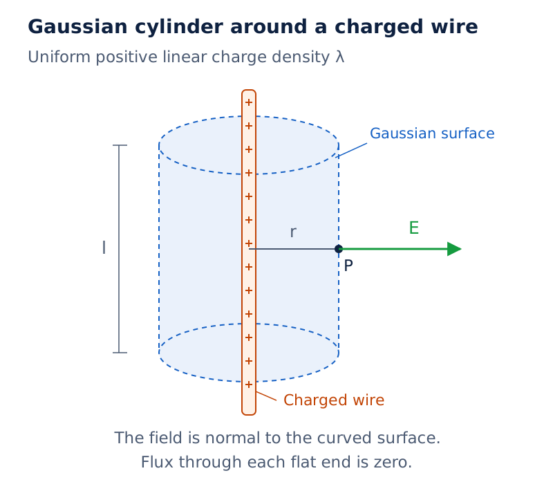
A vertical positively charged wire passes along the cylinder’s axis. The cylinder is labelled with radius and length, and a single outward horizontal field arrow E is drawn at a point P at distance r from the wire.

See Fig. 1.26 in your NCERT textbook

Derivation: Field of a line charge

Take a cylinder of radius $r$ and length $l$, with its axis on the wire.

1. Only the curved surface contributes: $$\Phi=E(2\pi rl).$$
2. The charge enclosed is $$Q_{\mathrm{enc}}=\lambda l.$$
3. Apply Gauss’s law: $$E(2\pi rl)=\frac{\lambda l}{\varepsilon_0}.$$
4. Cancel the length: $$\mathbf E=\frac{\lambda}{2\pi\varepsilon_0r}\hat{\mathbf n},$$ where $\hat{\mathbf n}$ is radially outward from the wire.

Wire result: The field points outward for positive linear charge density and inward for negative density. Its magnitude decreases inversely with radial distance. The scalar derivation above uses a positive charge density; the vector result includes either sign.

The infinite-length assumption supplies the required symmetry. For a finite long wire, the result is approximately valid near its central region when end effects are negligible. The field is due to the entire wire, although the flux relation uses only charge inside the Gaussian cylinder.

How is the field of a uniformly charged infinite plane sheet obtained?

For an infinite plane sheet with uniform surface charge density $\sigma$, symmetry requires a field perpendicular to the plane. At equivalent points on opposite sides, its magnitude is equal. Choose a closed box crossing the sheet, with two faces parallel to it.

The field is parallel to the side faces, so they contribute no flux. For a positively charged sheet, the field points outward on both sides, matching the outward normals of the two parallel end faces.

Derivation: Field of a plane sheet

Let each parallel end face have area $A$, equal to the sheet area enclosed by the box.

1. The end-face contributions add: $$\Phi=EA+EA=2EA.$$
2. The enclosed charge is $$Q_{\mathrm{enc}}=\sigma A.$$
3. Gauss’s law gives $$2EA=\frac{\sigma A}{\varepsilon_0}.$$
4. Cancel the area to obtain $$\mathbf E=\frac{\sigma}{2\varepsilon_0}\hat{\mathbf n},$$ with $\hat{\mathbf n}$ directed away from the sheet on the chosen side.

Sheet result: The field is independent of distance from an ideal infinite sheet. It points away for positive surface charge density and towards the sheet for negative density. The scalar steps above use positive density.

For a large finite sheet, this expression is an approximation in its middle region away from edges. The factor of two comes from flux through two faces; omitting one face incorrectly doubles the field.

Why is the field inside a uniformly charged spherical shell zero?

A thin spherical shell of radius $R$, uniformly charged with total charge $Q$, has spherical symmetry. Its field must be radial, with the same magnitude at all points equally far from its centre. Use a concentric spherical Gaussian surface.

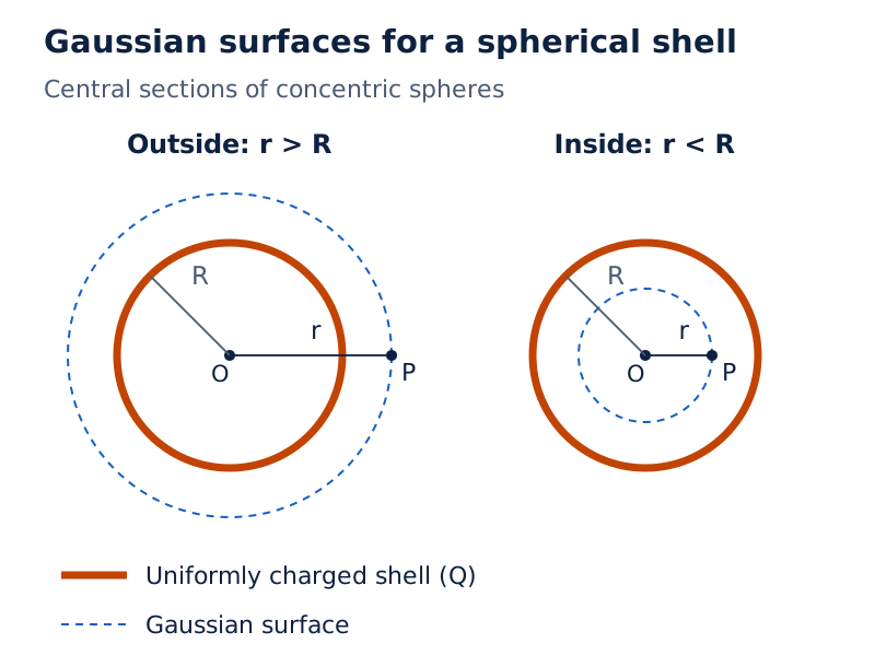
Two panels show the charged shell centred at the origin. One dashed Gaussian sphere passes through an exterior point; the other lies inside the shell. The shell radius and the observation point’s radial distance are separately labelled.

See Fig. 1.28 in your NCERT textbook

Derivation: Exterior and interior fields

First take a Gaussian radius greater than the shell radius, then one smaller than it.

1. Outside the shell, the enclosed charge is the full shell charge: $$Q_{\mathrm{enc}}=Q=4\pi R^2\sigma,\qquad r>R.$$
2. Using symmetry, $$E(4\pi r^2)=\frac{Q}{\varepsilon_0},\qquad\mathbf E=\frac{Q}{4\pi\varepsilon_0r^2}\hat{\mathbf r}.$$
3. Inside the shell, no shell charge is enclosed: $$Q_{\mathrm{enc}}=0,\qquad r<R.$$
4. The spherical flux relation then gives $$E(4\pi r^2)=0,\qquad\mathbf E=\mathbf0.$$ Symmetry also gives zero field at the centre.

Shell result: Outside, the field equals that of a point charge at the centre. Everywhere inside, it is zero. This conclusion uses both zero enclosed charge and spherical symmetry; zero enclosed charge alone is insufficient for an arbitrary arrangement.

Comparing the three symmetric distributions

In each application, identify the symmetry before simplifying the flux integral. A convenient surface makes either the normal field component constant or its contribution zero. Gauss’s law remains valid even when no such simple surface is available.

Glossary

• Electric charge — A property occurring in positive and negative forms, responsible for electric attraction and repulsion between charged bodies.
• Conductor — A material in which electric charges can move comparatively freely through the material.
• Insulator — A material offering high resistance to charge movement, so deposited charge remains localised.
• Point charge — An idealisation treating a charged body’s dimensions as negligible compared with the relevant separation.
• Charge conservation — The total electric charge of an isolated system remains unchanged despite internal redistribution.
• Charge quantisation — The occurrence of free charge in integral multiples of the elementary charge.
• Superposition principle — Individual electrostatic contributions remain unaffected by other charges and combine by vector addition.
• Electric field — Force per unit positive test charge at a point without disturbing the source arrangement.
• Electric field line — A directed curve whose tangent indicates the resultant electric field direction at each point.
• Electric flux — A scalar measure of electric field through a surface, accounting for area and orientation.
• Electric dipole — Two equal and opposite point charges separated by a finite distance from each other.
• Dipole moment — Charge magnitude multiplied by separation, directed from the negative towards the positive charge.
• Gaussian surface — An imaginary closed surface chosen to relate electric flux to the charge it encloses.
• Surface charge density — Charge per unit area, described macroscopically by averaging over many microscopic charged constituents.

Common errors and misconceptions

• Misconception: Rubbing produces new electric charge. Correct: Electrons transfer between bodies, while the total charge of the isolated system remains unchanged.
• Misconception: A neutral body has no charged particles. Correct: Its positive and negative charges balance, giving zero net charge.
• Misconception: The electric field points in the force direction for every charge. Correct: A negative charge experiences force opposite to the electric field.
• Misconception: Flux uses the angle between the field and the surface plane. Correct: The cosine uses the angle between the field and the surface normal.
• Misconception: A dipole has no field because its net charge is zero. Correct: Its separated charges generally produce a non-zero resultant field.
• Misconception: The distant axial dipole formula applies everywhere. Correct: For a finite dipole it requires distance much greater than the half-separation; points between the charges need separate treatment.
• Misconception: Zero flux proves the field is zero. Correct: It establishes zero net enclosed charge, while local fields can remain non-zero.
• Misconception: Only enclosed charges produce the field in Gauss’s law. Correct: All charges contribute to the field, but only enclosed charge determines its net closed-surface flux.

Exam-style questions with model answers

Q1. Explain conservation of charge when a glass rod is rubbed with silk. [2 marks]

1. Electrons transfer from the glass rod to the silk. The rod becomes positive and the silk negative.
2. The charges gained are equal and opposite, so the isolated rod-and-silk system retains its original net charge.

Q2. State Coulomb’s law in vector form and explain its signs and conditions. [3 marks]

1. For stationary point charges in vacuum, $\mathbf F_{21}=q_1q_2\hat{\mathbf r}_{21}/(4\pi\varepsilon_0r_{21}^2)$. Here $\mathbf F_{21}$ is the force on the second charge due to the first, and the unit vector points from the first charge towards the second.
2. A positive charge product gives a force along this direction, representing repulsion. A negative product reverses the direction and gives attraction.
3. The point-charge approximation requires body dimensions much smaller than separation. The mutual forces are equal and opposite, satisfying $\mathbf F_{12}=-\mathbf F_{21}$.

Q3. Explain three rules for electrostatic field lines. [3 marks]

1. A field line’s tangent gives the resultant field direction. Lines leave positive charges and enter negative charges, or extend to infinity for isolated charges.
2. Two lines cannot cross, because the field at a single point cannot have two different directions.
3. Electrostatic lines do not form closed loops. Their relative crowding represents field strength, while continuity is maintained through charge-free regions.

Q4. Derive the axial field of a finite dipole and obtain its distant-point form. [5 marks]

1. Take charges of magnitude $q$, separation $2a$, and dipole moment $\mathbf p=2qa\hat{\mathbf p}$. Choose a point on the axis beyond the positive charge, at distance $r>a$ from the centre.
2. The positive charge gives $\mathbf E_+=kq\hat{\mathbf p}/(r-a)^2$. The negative charge gives $\mathbf E_-=-kq\hat{\mathbf p}/(r+a)^2$. The two directions oppose.
3. Add the fields: $\mathbf E=kq[(r-a)^{-2}-(r+a)^{-2}]\hat{\mathbf p}$. The nearer positive charge gives the larger contribution.
4. Combining fractions gives $\mathbf E=4kqar\hat{\mathbf p}/(r^2-a^2)^2=2kpr\hat{\mathbf p}/(r^2-a^2)^2$.
5. For $r\gg a$, the denominator approaches $r^4$, so $\mathbf E\approx2k\mathbf p/r^3$. The field follows the dipole moment and decreases inversely with the cube of distance.

Q5. State Gauss’s law and explain why zero flux need not mean zero field. [3 marks]

1. Gauss’s law states $\oint\mathbf E\cdot\mathrm d\mathbf S=Q_{\mathrm{enc}}/\varepsilon_0$, with area vectors directed outward from the closed surface.
2. Zero net flux establishes zero algebraic enclosed charge. Positive and negative enclosed charges may cancel, or the surface may contain no charges.
3. External charges can still produce a field on the surface. In a uniform field, flux entering one end of a suitably aligned cylinder cancels the flux leaving the other.

Q6. Derive the electric field on both sides of a uniformly charged infinite plane sheet. [5 marks]

1. Let the uniform surface charge density be positive $\sigma$. By symmetry, the electric field is perpendicular to the plane, equal in magnitude on opposite sides and directed away from it.
2. Choose a closed box crossing the sheet. Each face parallel to the sheet has area $A$. The field is tangent to the other faces, giving zero side flux.
3. Both parallel faces have field along their outward normals, so $\Phi=EA+EA=2EA$.
4. The enclosed charge is $Q_{\mathrm{enc}}=\sigma A$. Gauss’s law gives $2EA=\sigma A/\varepsilon_0$, hence $E=\sigma/(2\varepsilon_0)$.
5. The result is independent of distance for the infinite sheet. For negative surface charge density the direction is towards the sheet, and the magnitude is $|\sigma|/(2\varepsilon_0)$. A finite large sheet approximates this behaviour away from its edges.

Q7. Why can a dipole experience torque but no net force in a uniform field? [2 marks]

1. The charges experience equal and opposite forces at different points. Their vector sum is zero, but they form a couple.
2. The torque is $\boldsymbol\tau=\mathbf p\times\mathbf E$, tending to align the dipole with the field.

Q8. Explain the fields inside and outside a uniformly charged thin spherical shell. [3 marks]

1. Spherical symmetry gives a radial field of constant magnitude on each concentric Gaussian sphere.
2. Outside, the sphere encloses the full charge. Gauss’s law gives $E(4\pi r^2)=Q/\varepsilon_0$, so the vector field equals $Q\hat{\mathbf r}/(4\pi\varepsilon_0r^2)$, as for a central point charge.
3. Inside, the enclosed charge is zero. Symmetry gives $E(4\pi r^2)=0$, hence zero field. The conclusion depends on symmetry as well as zero enclosed charge.

Key takeaways

• Charging by friction transfers electrons between bodies; it does not create net charge in an isolated system.
• Charge is additive, conserved and quantised, although microscopic steps can be ignored in many macroscopic calculations.
• Coulomb’s law gives individual forces; superposition combines their vectors while retaining directions and charge signs.
• The electric field belongs to the source arrangement, while the force also depends on the test charge.
• Electric flux uses the surface normal, and outward normals fix signs when the surface is closed.
• A dipole has zero total charge but generally a non-zero field, with inverse-cube decay at large distances.
• A uniform external field produces no net dipole force, but it can produce an aligning torque.
• Gauss’s law relates flux to enclosed charge; symmetry makes it useful for calculating wire, sheet and shell fields.

Test yourself

Why does a glass rod become positive when rubbed with silk?

Some electrons transfer from glass to silk, leaving the rod with an electron deficit.

What does the integer in the charge-quantisation relation represent?

In $q=ne$, the signed integer counts elementary charge units making up the body’s net charge.

What is the force direction on an electron in an electric field?

Because the electron has negative charge, its force points opposite to the electric field.

Why can two electrostatic field lines not cross?

A crossing would require two distinct electric field directions at one point, which is not possible.

When is flux through a small planar element zero despite a non-zero field?

It is zero when the field is tangent to the element, perpendicular to its area vector.

Which way does a dipole’s equatorial field point?

It points opposite to the dipole moment, whose direction is from negative to positive charge.

Can charges outside a Gaussian surface affect the field on it?

Yes. They contribute to the local field, but not to the net closed-surface flux.

Why does the infinite-sheet field lack a distance factor?

Gauss's law gives $2EA=\sigma A/\varepsilon_0$, in which distance never appears: the same $E=\sigma/(2\varepsilon_0)$ results wherever the two end faces are placed, because the enclosed charge $\sigma A$ and the end-face area $A$ do not depend on how far the faces are from the sheet.