
Linear Programming | CBSE Class 12 Maths Notes
On this page
Linear Programming in Mathematics covers optimisation, decision variables, objective functions, linear constraints, feasible regions, the graphical method, corner-point evaluation, bounded and unbounded regions, multiple optimal solutions and problems with no feasible solution.
What does a linear programming problem ask us to find?
An optimisation problem seeks a best possible outcome, such as maximum profit, minimum cost or minimum use of resources. A linear programming problem is a special kind of optimisation problem in which the objective and the restrictions are linear.
The task has two connected parts: describe the choices allowed by the restrictions, then identify the allowed choice giving the greatest or smallest objective value. A choice that gives an attractive profit but breaks a restriction cannot solve the problem.
What are decision variables and the objective function?
Decision variables represent the quantities to be chosen. Let and denote two such quantities. Let denote the value to be maximised or minimised, and let and denote fixed coefficients.
Definition: A linear objective function has the form . Its optimal value is its maximum or minimum value under the given constraints.
The letters acquire their practical meanings from the problem. In the furniture problem, the variables count tables and chairs, while the objective measures profit. In a purely graphical problem, the variables may simply be the coordinates used to describe the feasible region.
What does linear programming mean?
Linear refers to the linear mathematical relations used in the problem. Programming refers to determining a programme or plan of action. Here the method is graphical: draw the restrictions in two variables, locate their common region and evaluate the objective appropriately.
Constraints are the equations, inequalities or restrictions on the variables. Non-negative restrictions are included among them. An objective function alone does not specify a complete problem: the direction of optimisation and the full set of constraints must also be stated.
How is the furniture dealer's problem formulated?
A furniture dealer has ₹50,000 to invest and space for at most 60 pieces. A table costs ₹2,500 and a chair costs ₹500. The profit is ₹250 per table and ₹75 per chair. Assume that all purchased items can be sold.
Let be the number of tables purchased and the number of chairs purchased. Let be the total profit in rupees. The dealer wants to choose the purchases that give the greatest profit while respecting both investment and storage limits.
How do the words become inequalities?
- Step 1: Non-negativity. Numbers of purchased items cannot be negative:
- Step 2: Investment. Multiply each quantity by its purchase price, then compare the total with the available capital:
- Step 3: Simplification. Divide the investment inequality by the positive number 500:
- Step 4: Storage. Both kinds of furniture occupy places in the total allowance:
- Step 5: Objective. Add the profits from the two purchases: Maximise this expression subject to all four restrictions.
The phrase at most permits using less than the available amount. It therefore produces an inequality rather than a requirement that all capital or all storage must be used. The boundary equation is useful for drawing, but the inequality represents the permitted side.
| Part of the model | Mathematical statement | Meaning |
|---|---|---|
| Investment | Purchases remain within the available money. | |
| Storage | The combined number fits the storage space. | |
| Non-negativity | Neither purchase quantity is negative. | |
| Objective | Maximise | Compare total profit among feasible purchases. |
Formulation must keep purchase costs separate from profits. The prices belong in the investment constraint; the profits belong in the objective function. Exchanging them would describe a different problem even if the resulting graph were drawn correctly.
How do feasible regions and feasible solutions differ?
The feasible region is the common region satisfying every constraint, including non-negativity. Each inequality selects a half-plane. Intersecting all those half-planes gives the set of choices that the problem actually permits.
A feasible solution is a point within or on the boundary of this region. An infeasible solution lies outside it. The distinction concerns all restrictions together: satisfying just the investment condition or just the storage condition is insufficient.
How can a proposed solution be checked?
For the furniture model, check the given feasible point , where the first coordinate counts tables and the second counts chairs. Also compare the point , which is infeasible.
- Step 1: For the first point, the investment expression is It satisfies the investment constraint at equality.
- Step 2: Its storage expression is Both coordinates are non-negative, so every restriction is satisfied.
- Step 3: For the second point, investment requires a bound of 100, but
- Step 4: Its total number of items is also excessive: It lies outside the feasible region.
An optimal feasible solution does more than meet the constraints: it gives the required maximum or minimum of the objective. A feasible point may therefore be acceptable without being best. Testing feasibility and testing optimality answer different questions.
What is a corner point?
A corner point, also called a vertex, is the intersection of two boundary lines that belongs to the feasible region. Intersections outside the common region are excluded. The furniture region has four vertices, which will provide a finite set of candidates for maximising profit.
Why can the graphical method focus on corner points?
Let denote the feasible region. Continue to use , where is the objective value, and are decision variables, and and are constants. Corner-point results connect the region's geometry with optimisation.
Theorem: An existing optimum occurs at a vertex
If the objective has an optimal value on the feasible region, that value occurs at a corner point. This is an existence-conditioned statement. It identifies where an optimum can be found when an optimum exists; it does not guarantee one for every unbounded problem.
Theorem: A bounded feasible region has both extrema
For a non-empty bounded feasible region, the objective has both a maximum and a minimum, each attained at a corner point. A region is bounded if it can be enclosed within a circle. An unbounded region extends indefinitely in some direction.
Result: Equal optimal corner values give multiple optima
If two corner points give the same maximum value, every point on the line segment joining them gives that maximum. The corresponding statement holds for a shared minimum. Thus a corner-point optimum need not be the only optimal solution.
What are the steps of the corner-point method?
- Locate the region. Graph all constraints and identify their common feasible region, including the coordinate restrictions.
- Find the vertices. Read obvious intercepts or solve the simultaneous boundary equations. Retain intersections that satisfy all constraints.
- Evaluate the objective. Calculate its value at every corner. Let be the largest corner value and the smallest corner value.
- Check boundedness. For a bounded feasible region, these are the maximum and minimum. For an unbounded region, perform the additional half-plane test.
For an unbounded region, is a maximum if the open half-plane has no common point with the feasible region. Similarly, is a minimum if has no common point with it.
Note: A table of corner values completes a bounded problem. In an unbounded problem, the same table gives candidates whose optimality still needs checking.
How does the dealer obtain the maximum profit?
The furniture model provides a complete example of bounded optimisation. The restrictions on money and storage cut out a finite region in the first quadrant. The two sloping boundaries meet at the purchase combination where both resources are fully used.
Worked example 1. Maximise profit , where counts tables and counts chairs, subject to , , and .
- Step 1: Axis vertices. On the horizontal axis, , so investment gives and hence . On the vertical axis, , and storage gives . Include the origin .
- Step 2: Boundary intersection. Subtract the storage boundary from the investment boundary:
- Step 3: Second coordinate. Substitute into the storage boundary: Thus the fourth vertex is .
- Step 4: Objective values. At the four corners calculate
- Step 5: Compare. The region is bounded, and the largest corner value is , attained at .
Answer: Buy 10 tables and 50 chairs for a maximum profit of ₹6,250.
What the figure shows
Furniture choices
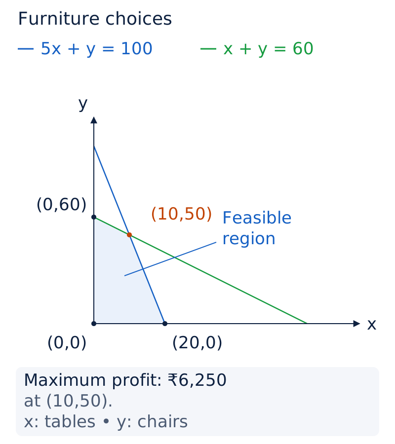
The blue feasible region lies in the first quadrant, bounded by the axes and the lines and . Its labelled non-origin vertices are , and .
Drawn by One Young India. See Fig. 12.1 in your NCERT textbook
How is the purchase plan checked?
- Step 1: Investment check.
- Step 2: Storage check.
- Step 3: Profit check.
The notation means the objective value obtained by substituting that ordered pair. It does not represent a new restriction. Keeping the coordinates beside each computed value helps connect the arithmetic to the corresponding purchase plan.
The practical answer states both the quantities and the profit. A number alone would omit the investment strategy the dealer needs. Here the optimal plan uses the entire capital and storage allowance, as the final checks confirm.
How is a bounded maximisation problem solved?
A graphical problem may supply its objective and constraints directly. In that case the modelling has already been done, but the reasoning still requires a feasible region, its vertices and a comparison of objective values. The intersection of the sloping lines is not automatically optimal.
Worked example 2. Let and be decision variables and the objective value. Maximise subject to , , and .
- Step 1: Axis limits. Setting gives the tighter horizontal limit . Setting gives the tighter vertical limit . The origin satisfies all constraints.
- Step 2: Intersection. Solve the two boundary equations by subtraction:
- Step 3: Complete the point. The vertices are , , and .
- Step 4: Evaluate.
- Step 5: Select. The feasible region is bounded. Its largest corner value is , which occurs at .
Answer: The maximum value is at .
What the figure shows
Bounded maximisation
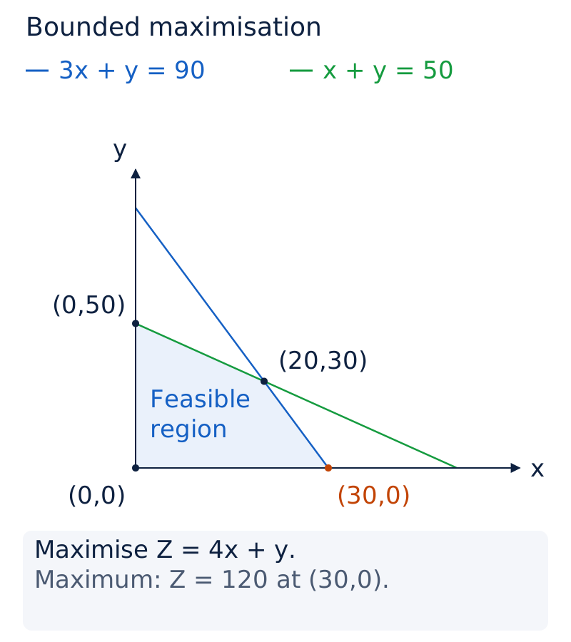
The graph shades the first-quadrant region below both sloping boundaries. It labels the feasible corners , and , together with the origin.
Drawn by One Young India. See Fig. 12.2 in your NCERT textbook
Why does the intersection not win?
The objective attaches different coefficients to the two variables. Although lies on both sloping boundaries, its objective value is smaller than the value at . The objective comparison, rather than the appearance of the graph, decides which corner is best.
Axis intercepts must also be checked against the other inequality. An intercept belonging to one boundary line can lie outside the feasible region. The correct vertex list records the limits permitted by the whole system, not every intercept used while drawing individual lines.
How does minimisation work when inequalities face different ways?
A lower-bound condition and an upper-bound condition can enclose a bounded feasible region together. Do not assume that the origin belongs to every problem in the first quadrant. It must satisfy the original inequalities just as any other candidate point must.
Worked example 3. Let and be decision variables and the objective value. Minimise subject to , , and .
- Step 1: Vertical vertices. With , the inequalities require and . The vertical boundary therefore contributes and .
- Step 2: Eliminate a variable. Double the first boundary equation to obtain . Subtract this from the second:
- Step 3: Find the intersection. The third vertex is .
- Step 4: Evaluate each corner.
- Step 5: Conclude. The triangular feasible region is bounded. The smallest corner value is .
Answer: The minimum value is at .
What the figure shows
Bounded minimisation
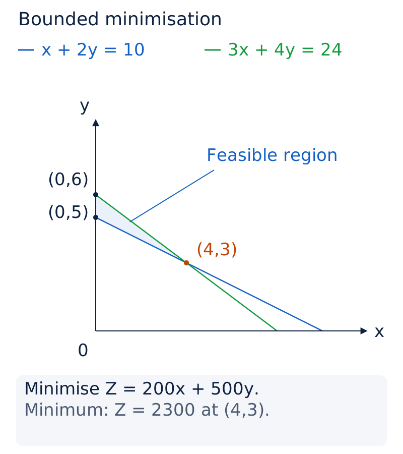
The small shaded triangle has labelled vertices , and . Its sloping sides lie on and .
Drawn by One Young India. See Fig. 12.3 in your NCERT textbook
What does the inequality direction change?
The first constraint selects the side at or above its boundary in this graph, while the second selects the side at or below its boundary. Their common region, together with non-negativity, is the triangle between the three feasible vertices.
The lower bound excludes the origin. Including it would introduce a false objective value smaller than the true minimum. Drawing the selected half-planes and checking the final vertices prevents this error. Minimisation uses the same corner-point framework as maximisation, with the comparison reversed.
How can a problem have more than one optimal solution?
The largest objective value may appear at two corners. This does not mean there are only two optimal solutions. When the corners share the optimum, the segment joining them also shares it. The graph therefore identifies a whole set of equally good choices.
Worked example 4. Let and be decision variables and the objective value. Minimise and maximise subject to , , , and .
- Step 1: Vertical corners. With , the active limits give and . Call these vertices and .
- Step 2: Lower diagonal corner. On the boundary , the equation becomes . Hence , giving .
- Step 3: Upper diagonal corner. On the same boundary, becomes . Hence , giving .
- Step 4: Compare values.
- Step 5: Identify the whole maximum set. Along the feasible segment joining and ,
Answer: The minimum is at . The maximum is at every point on the segment from to .
What the figure shows
Multiple optimal solutions
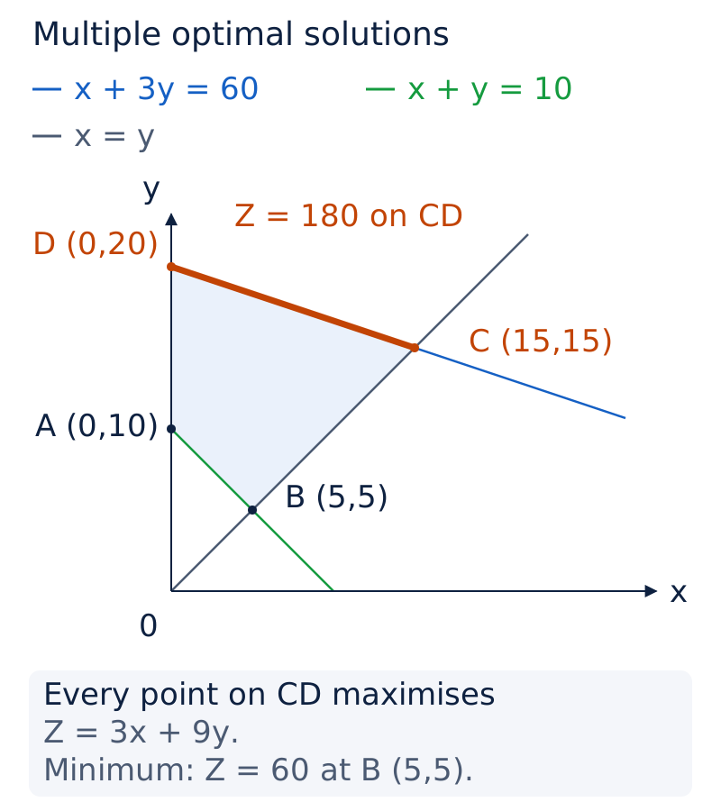
The shaded quadrilateral has vertices , , and . The upper sloping side joins the two corners whose objective values are both .
Drawn by One Young India. See Fig. 12.4 in your NCERT textbook
What must be stated in the conclusion?
Separate the optimal value from the optimal solutions. The maximum value is a single number, but the coordinate pairs that produce it are multiple. Naming only the two end points would leave out the other optimal points on their joining segment.
The expression for the objective explains the equality directly: it is three times the boundary expression. This calculation confirms the geometric result without checking an endless list of individual points. The segment remains inside the feasible region, so these equal objective values are attainable.
Why does an unbounded region need an extra test?
An unbounded feasible region continues indefinitely. Its vertices provide useful candidate values, but they do not by themselves settle whether a maximum or minimum exists. The objective can take better values farther into the region than those recorded at the corners.
Worked example 5. Let and be decision variables and the objective value. Minimise , subject to , , , and .
- Step 1: Vertical boundary. At , the first two inequalities give and . Thus the vertical vertices are and .
- Step 2: Horizontal boundary. At , the second and third inequalities give and . Thus the horizontal vertices are and .
- Step 3: Corner values.
- Step 4: Test the candidate. The region is unbounded, so draw the open half-plane This half-plane has points in common with the feasible region.
- Step 5: Decide. The extra test rejects as a minimum. The objective has no minimum value under the stated constraints.
Answer: There is no minimum value; is only the smallest value among the corners.
What does the graph test establish?
The test asks whether feasible points can lie on the side giving a value strictly smaller than the candidate. The strict inequality matters: points on the equal-value line do not improve the objective. The open half-plane represents values beyond that line.
What the figure shows
Unbounded feasible region
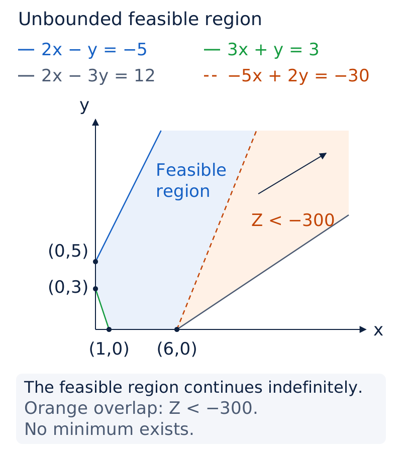
The blue region extends to the right beyond the four labelled corners. A dashed line labelled passes through the region, illustrating the extra test for the candidate minimum.
Drawn by One Young India. See Fig. 12.5 in your NCERT textbook
Unbounded region and no minimum are not interchangeable statements. Some unbounded problems do have a minimum. The absence of a minimum here follows from the additional test for this objective and these constraints, not from the word unbounded alone.
What happens when the constraints have no common region?
A linear programming problem may have no feasible solution. This means there is no point satisfying all the restrictions simultaneously. Calculating objective values at selected boundary intersections cannot repair that failure, because the proposed choices are not permitted by the complete system.
Worked example 6. Let and be decision variables and the objective value. Minimise , subject to , , and .
- Step 1: First boundary. The line meets the axes at and . Select the half-plane satisfying the greater-than-or-equal restriction.
- Step 2: Second boundary. The line meets the axes at and . Select the half-plane satisfying the less-than-or-equal restriction.
- Step 3: Algebraic check. From and , obtain
- Step 4: Contradiction. The same expression is required to be at most 15. Since , no point can satisfy both requirements.
Answer: There is no feasible or optimal solution: the constraints would require the same expression to be at least and at most .
How is infeasibility different from an unbounded objective?
In the preceding unbounded example, feasible points existed but there was no minimum. Here feasibility fails first. The distinction is essential: one conclusion concerns how the objective behaves on an existing region; the other concerns the absence of that region.
What the figure shows
Incompatible half-planes
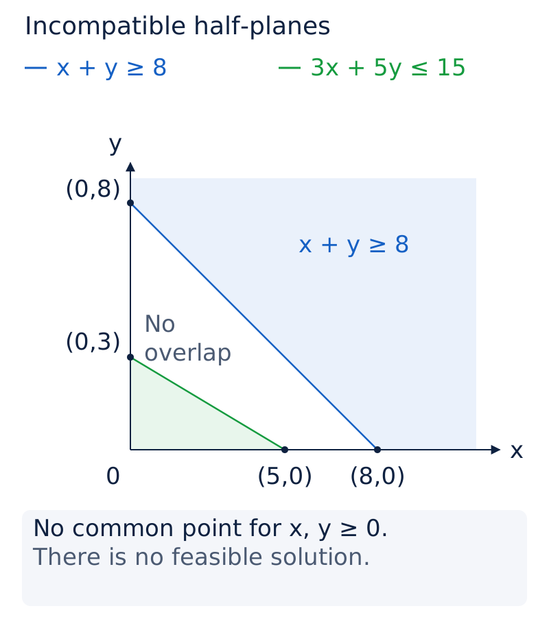
The graph labels the intercepts , , and . The selected regions for the two sloping boundaries do not overlap in the first quadrant.
Drawn by One Young India. See Fig. 12.6 in your NCERT textbook
How do further examples bring the method together?
The same procedure handles a simple triangular region and an unbounded region with multiple minima. These cases help separate the shape of the feasible set from the behaviour of the objective. First identify the region; then apply the appropriate optimisation argument.
How is a single-constraint maximum found?
Worked example 7. Let and be decision variables and the objective value. Maximise , subject to , and .
- Step 1: Draw the boundary. The equation has intercepts and .
- Step 2: Select the region. Together with non-negativity, the inequality gives the bounded triangle with vertices , and .
- Step 3: Evaluate.
- Step 4: Compare. The largest corner value is , so it is the maximum on the bounded region.
Answer: The maximum is at .
Can an unbounded region have multiple minima?
Worked example 8. Let and be decision variables and the objective value. Minimise , subject to , , and . Show that more than two points give the minimum.
- Step 1: Identify a lower bound. One constraint is already the objective expression: Therefore no feasible point can give a smaller value.
- Step 2: Locate the equal-value segment. The line meets the axes at and . On the segment between these points,
- Step 3: Check the other constraint. Substitution along this segment gives Both coordinates are non-negative there.
- Step 4: Evaluate the whole segment. The lower bound is attained at every point of the segment.
Answer: The minimum is , attained throughout the segment from to , giving more than two optimal points.
The final example also completes the open-half-plane test directly. The condition cannot share a point with the feasible region, because it contradicts one of the original constraints. Thus the unbounded region has an attained minimum.
Glossary
- Linear programming problem — A problem optimising a linear objective while satisfying linear constraints and non-negative restrictions.
- Optimisation — Finding a maximum or minimum value while respecting the restrictions imposed on the choices.
- Decision variables — Quantities whose values are chosen to determine a feasible plan and its objective value.
- Objective function — The linear function whose maximum or minimum value is required under the given constraints.
- Constraints — Equations, inequalities or restrictions that the variables of a linear programming problem must satisfy.
- Non-negative restrictions — Conditions requiring the decision variables to be zero or positive rather than negative.
- Feasible region — The common region satisfying every constraint, including the restrictions that variables are non-negative.
- Feasible solution — A point within or on the boundary of the region satisfying all constraints.
- Infeasible solution — A point outside the feasible region because it fails to satisfy the full constraint system.
- Optimal solution — A feasible point giving the required maximum or minimum value of the objective function.
- Corner point — A vertex in the feasible region formed by the intersection of two boundary lines.
- Bounded region — A feasible region that can be enclosed completely within a circle.
- Unbounded region — A feasible region that extends indefinitely and cannot be enclosed within a circle.
- Multiple optimal solutions — More than one feasible point giving the same required maximum or minimum objective value.
Common errors and misconceptions
- Misconception: Any point satisfying one inequality is feasible. Correct: A feasible point must satisfy every constraint, including non-negativity.
- Misconception: Only points strictly inside the region are feasible. Correct: Points on its included boundaries are feasible too.
- Misconception: The intersection of the sloping boundaries must be optimal. Correct: Evaluate the objective at all feasible corners before comparing values.
- Misconception: An unbounded region cannot have a minimum. Correct: A minimum may exist; test whether any feasible point lies in the improving open half-plane.
- Misconception: The smallest corner value proves a minimum in every problem. Correct: An unbounded region requires the additional half-plane check.
- Misconception: Two equally optimal corners mean exactly two optimal solutions. Correct: Every point on their joining segment gives the same optimum.
- Misconception: An empty feasible region means the objective value is zero. Correct: It means no feasible solution exists, so there is no optimal solution.
Exam-style questions with model answers
Q1. Distinguish a feasible solution from an optimal solution in linear programming. [2 marks]
- A feasible solution is any point within or on the boundary of the region satisfying all constraints.
- An optimal solution is a feasible point that also gives the required maximum or minimum value of the objective function.
Q2. A dealer has ₹50,000 and storage for 60 pieces. Tables cost ₹2,500 each and chairs ₹500 each. Profits are ₹250 and ₹75 respectively, and all purchases can be sold. Formulate the profit-maximisation problem. [3 marks]
- Let count tables, count chairs and represent profit in rupees. The quantities cannot be negative, so and .
- The purchase expenditure cannot exceed the investment: , or .
- The combined storage requirement gives . Total profit is . Maximise this function subject to the investment, storage and non-negative constraints together.
Q3. Maximise subject to , , and , where are decision variables and is the objective value. Show the corner-point calculations. [5 marks]
- The non-negative constraints restrict the region to the first quadrant. On the horizontal axis, the tighter bound is ; on the vertical axis it is . The origin is also feasible.
- Subtract the boundary equations: , so and . Then .
- The common region is bounded, with vertices , , and .
- Evaluate the objective at each: , , and .
- The largest of these values is . The bounded-region theorem therefore gives a maximum of at . Both the optimum and the point producing it are required in the conclusion.
Q4. Minimise subject to , , and , where are decision variables and is the objective value. [4 marks]
- On the vertical axis the constraints give vertices and . For the sloping-line intersection, double , giving .
- Subtract from to obtain . Substitution gives , so .
- The bounded triangular region has corners , and . Their objective values are , and , respectively.
- The minimum is therefore at .
Q5. A bounded feasible region has vertices , , and . Find the minimum and maximum of , where are coordinates and is the objective value. Describe all maximum solutions. [4 marks]
- Evaluate the objective at the vertices: , , and .
- Because the region is bounded, the smallest and largest corner values are the extrema. The minimum is at .
- The maximum is . Both and attain it.
- Every point on their joining segment is also optimal. Along that segment, , giving .
Q6. Explain why the problem of minimising subject to , , and has no feasible solution. Here are decision variables and is the objective value. [3 marks]
- Begin with the lower bound . Multiplying by three gives .
- Since , adding cannot decrease that expression. Thus .
- This contradicts the required upper bound . No coordinate pair can satisfy the constraints simultaneously. Hence the common feasible region is empty, and there is no feasible solution or minimum objective value.
Key takeaways
- A linear programming problem optimises a linear objective subject to linear constraints and non-negative restrictions on its decision variables.
- The feasible region is the common part of all constraint regions, including its permitted boundary points.
- For a non-empty bounded feasible region, both extrema exist and can be found by comparing objective values at its corners.
- In an unbounded region, candidate corner values require an additional open-half-plane test before an optimum can be claimed.
- If two corners share an optimal value, every point on the segment joining them shares that value.
- No common feasible region means no feasible solution, which differs from an existing region with an unbounded objective.
- In a practical problem, report both the optimal decision-variable values and the resulting objective value with its meaning.
Test yourself
What does the word programming mean in this chapter?
It means determining a particular programme or plan of action under the given restrictions.
Must a feasible solution lie strictly inside the feasible region?
No. Points on the boundary also represent feasible solutions when they satisfy every constraint.
How is a bounded feasible region defined?
It is a feasible region that can be enclosed within a circle.
Why is the largest corner value insufficient in an unbounded maximisation problem?
Other feasible points may give larger values. Check the open half-plane where the objective exceeds that candidate.
What follows if two corners give the same minimum value?
Every point on the line segment joining those corners gives the same minimum value.
What is the first conclusion when all constraint half-planes have no common point?
The problem has no feasible region and therefore no feasible solution.
Can an unbounded feasible region still have an attained minimum?
Yes. A minimum can exist if the open half-plane giving smaller objective values contains no feasible points.
Write about it
Turn a question from this chapter into a paper.
The Writing Studio has a structure guide, a rubric and citation tools for 15 formats, from essays to research papers. Drafting is free with an account. Learnacy Essential adds feedback from an AI writing coach and submission to The OYI Review.
Learnacy Essential is ₹1,499 for the year. Publication depends on review and is not guaranteed.