Statistics | CBSE Class 11 Maths Notes

This Class 11 Mathematics note covers measures of dispersion, range, mean deviation about the mean and median, variance, standard deviation, frequency distributions, step-deviation calculations, changes of origin and scale, missing observations, and correction of incorrectly recorded data.

Why do we need dispersion as well as an average?

Statistics deals with data collected for specific purposes and with its analysis and interpretation. Tables and graphs reveal features of data. A measure of central tendency, such as the mean, median or mode, indicates where the observations are centred.

An average alone does not describe how closely the observations cluster around that centre. Two sets can have the same mean and median but very different spreads. Dispersion describes this variability, supplying information that a central value leaves out.

How can equal averages hide different performances?

Consider the runs in ten matches. Batsman A scored $30,91,0,64,42,80,30,5,117,71$; batsman B scored $53,46,48,50,53,53,58,60,57,52$. Both have mean and median $53$. However, A's scores extend from $0$ to $117$, while B's extend from $46$ to $60$.

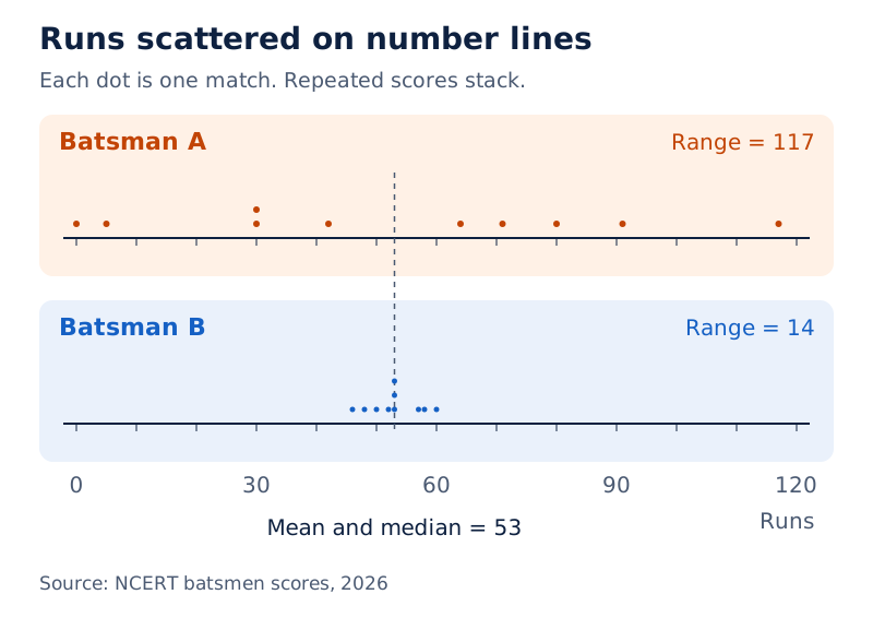
The upper number line shows A's scores spread widely, including dots at the low and high ends. The lower number line shows B's dots clustered close together around the central scores.

See Figs. 13.1 and 13.2 in your NCERT textbook

What does the range measure?

Definition: The range is the difference between the maximum and minimum observations. It gives a rough indication of scatter but does not measure deviations from a central value.

The calculation is $$\text{Range}=\text{maximum value}-\text{minimum value}.$$

1. For batsman A, subtract the smallest score from the largest: $$\text{Range of A}=117-0=117.$$
2. For batsman B, use the same subtraction: $$\text{Range of B}=60-46=14.$$
3. Compare the results: $$117>14.$$ A's scores are more dispersed by this measure, despite the identical central values.

The main measures considered here are range, mean deviation and standard deviation, together with variance. Mean deviation and standard deviation use distances or deviations from a central value, allowing the calculation to take account of more than the two extreme observations.

How is mean deviation calculated for ungrouped data?

Let $n$ be the number of observations and $x_i$ the observation at position $i$, where $i$ is an index running from $1$ to $n$. The symbol $\sum$ means that the indicated quantities are added. Write $\bar{x}$ for the arithmetic mean and $M$ for the median.

Let $a$ denote the central value about which deviations are measured. A deviation is $x_i-a$. Its absolute value, $|x_i-a|$, is the distance from the centre, with any negative sign removed. Absolute values prevent positive and negative deviations from cancelling.

Definition: Mean deviation about a central value is the arithmetic mean of the absolute deviations from it. The notation $\mathrm{MD}(a)$ means mean deviation about $a$: $$\mathrm{MD}(a)=\frac{1}{n}\sum_{i=1}^{n}|x_i-a|.$$

First calculate the required centre, then subtract it from each observation, take absolute values, and average those values. For the mean, use $\bar{x}=\frac{1}{n}\sum_{i=1}^{n}x_i$. For the median, arrange the data in order before locating the middle.

How do we use the mean as the centre?

Worked example 1. Find the mean deviation about the mean for $6,7,10,12,13,4,8,12$.

Answer: Calculate the mean before forming the deviations.

1. Add all eight observations and divide by their number: $$\bar{x}=\frac{6+7+10+12+13+4+8+12}{8}=\frac{72}{8}=9.$$
2. Subtract the mean in the original observation order: $$(6-9,7-9,10-9,12-9,13-9,4-9,8-9,12-9)=(-3,-2,1,3,4,-5,-1,3).$$
3. Take absolute values and add: $$\sum_{i=1}^{8}|x_i-9|=3+2+1+3+4+5+1+3=22.$$
4. Divide by the observation count: $$\mathrm{MD}(\bar{x})=\frac{22}{8}=2.75.$$

How do we use the median as the centre?

For an odd observation count, the median occupies position $(n+1)/2$ in the ordered data. For an even count, average the observations in positions $n/2$ and $n/2+1$. These are positions, not numbers to substitute as the median.

Worked example 2. Find the mean deviation about the median for $3,9,5,3,12,10,18,4,7,19,21$.

Answer: Order the eleven observations and locate the middle value.

1. Arrange the data: $$3,3,4,5,7,9,10,12,18,19,21.$$
2. The median position is $(11+1)/2=6$, so $M=9$.
3. Subtract the median from the ordered values and take absolute values: $$|x_i-9|:\quad6,6,5,4,2,0,1,3,9,10,12.$$
4. Add and divide by eleven: $$\mathrm{MD}(M)=\frac{6+6+5+4+2+0+1+3+9+10+12}{11}=\frac{58}{11}\approx5.27.$$

Mean deviation about the mean and mean deviation about the median are distinct calculations. The chosen centre must remain the same throughout the deviation column. Replacing one centre with the other partway through changes the quantity being calculated.

How do frequencies change a mean-deviation calculation?

A discrete frequency distribution records distinct values and the number of times each occurs. Let $f_i$ denote the frequency of value $x_i$, and let $N$ denote the total frequency. Here $n$ counts distinct values, whereas $N=\sum_{i=1}^{n}f_i$ counts all observations.

Each value contributes to the sum as many times as it occurs. Therefore, calculate the weighted mean as $\bar{x}=\frac{1}{N}\sum_{i=1}^{n}f_ix_i$. Apply the same frequency weighting to absolute deviations, giving $\mathrm{MD}(a)=\frac{1}{N}\sum_{i=1}^{n}f_i|x_i-a|$.

How is mean deviation about the mean tabulated?

Worked example 3. Find mean deviation about the mean for the values and frequencies in the first two columns.

Answer: The remaining columns show the products and distances used in the calculation.

Value $x_i$	Frequency $f_i$	Product $f_ix_i$	Distance $|x_i-7.5|$	Weighted distance $f_i|x_i-7.5|$
$2$	$2$	$4$	$5.5$	$11$
$5$	$8$	$40$	$2.5$	$20$
$6$	$10$	$60$	$1.5$	$15$
$8$	$7$	$56$	$0.5$	$3.5$
$10$	$8$	$80$	$2.5$	$20$
$12$	$5$	$60$	$4.5$	$22.5$

1. Add frequencies: $N=2+8+10+7+8+5=40$.
2. Add the products and calculate the mean: $$\bar{x}=\frac{4+40+60+56+80+60}{40}=\frac{300}{40}=7.5.$$
3. Subtract $7.5$, take absolute values and multiply by frequencies, as shown in the last two columns. Their weighted sum is $11+20+15+3.5+20+22.5=92$.
4. Average the weighted distances: $$\mathrm{MD}(\bar{x})=\frac{92}{40}=2.3.$$

How do cumulative frequencies locate the median?

Cumulative frequency is the running total of frequencies up to a value in ascending order. It locates an observation by its position without writing out every repeated value. For an even total, check the two central observations before taking their average.

Worked example 4. Find mean deviation about the median for these values and frequencies.

Answer: Use cumulative frequency to find the centre, then weight each absolute deviation.

Value $x_i$	Frequency $f_i$	Cumulative frequency	Distance $|x_i-13|$	Weighted distance
$3$	$3$	$3$	$10$	$30$
$6$	$4$	$7$	$7$	$28$
$9$	$5$	$12$	$4$	$20$
$12$	$2$	$14$	$1$	$2$
$13$	$4$	$18$	$0$	$0$
$15$	$5$	$23$	$2$	$10$
$21$	$4$	$27$	$8$	$32$
$22$	$3$	$30$	$9$	$27$

1. The last cumulative frequency gives $N=30$, so use the fifteenth and sixteenth observations.
2. Both positions fall after cumulative frequency $14$ and within cumulative frequency $18$: $$M=\frac{13+13}{2}=13.$$
3. Calculate each distance from $13$, multiply by its frequency, and add: $$\sum_{i=1}^{8}f_i|x_i-M|=30+28+20+2+0+10+32+27=149.$$
4. Divide by total frequency: $$\mathrm{MD}(M)=\frac{149}{30}\approx4.97.$$

Frequency weighting belongs in both the mean and deviation calculations. Dividing by the number of table rows would treat each distinct value as if it occurred once, losing the information supplied by the frequencies.

How is mean deviation found for continuous grouped data?

A continuous frequency distribution groups observations into class intervals without gaps. For calculations, assume that the frequency in each class is concentrated at its midpoint. Use those midpoints as the values $x_i$, and then apply the frequency formulas.

A midpoint is obtained by averaging the two class limits. This gives a representative value for each interval, rather than recovering the individual observations within it. Both the mean and the absolute-deviation columns must use the same set of midpoints.

How are class midpoints used about the mean?

Worked example 5. Find mean deviation about the mean for this distribution of marks.

Answer: Replace each class by its midpoint before computing the mean.

Marks interval	Students $f_i$	Midpoint $x_i$	Product $f_ix_i$	Distance $|x_i-45|$	Weighted distance
10 to 20	$2$	$15$	$30$	$30$	$60$
20 to 30	$3$	$25$	$75$	$20$	$60$
30 to 40	$8$	$35$	$280$	$10$	$80$
40 to 50	$14$	$45$	$630$	$0$	$0$
50 to 60	$8$	$55$	$440$	$10$	$80$
60 to 70	$3$	$65$	$195$	$20$	$60$
70 to 80	$2$	$75$	$150$	$30$	$60$

1. Average the limits of each class; for the first class, $x_1=(10+20)/2=15$. The other midpoints follow in the table.
2. Add frequencies and weighted values: $$N=2+3+8+14+8+3+2=40,\qquad\sum_{i=1}^{7}f_ix_i=30+75+280+630+440+195+150=1800.$$
3. Calculate $\bar{x}=1800/40=45$, then obtain the distance and weighted-distance columns.
4. Add those weighted distances and divide: $$\mathrm{MD}(\bar{x})=\frac{60+60+80+0+80+60+60}{40}=\frac{400}{40}=10.$$

How is the median found inside a class?

Identify the median class using cumulative frequencies and the position $N/2$. Let $l$ be its lower limit, $f$ its frequency, $h$ its width, and $C$ the cumulative frequency of the preceding class. The grouped median formula is $$M=l+\frac{N/2-C}{f}\,h.$$

Worked example 6. Calculate mean deviation about the median for the following distribution.

Answer: Find the median from cumulative frequencies, then measure midpoint distances from it.

Class	Frequency $f_i$	Cumulative frequency	Midpoint $x_i$	Distance $|x_i-28|$	Weighted distance
0 to 10	$6$	$6$	$5$	$23$	$138$
10 to 20	$7$	$13$	$15$	$13$	$91$
20 to 30	$15$	$28$	$25$	$3$	$45$
30 to 40	$16$	$44$	$35$	$7$	$112$
40 to 50	$4$	$48$	$45$	$17$	$68$
50 to 60	$2$	$50$	$55$	$27$	$54$

1. The total is $N=50$, giving $N/2=25$. The cumulative frequency first reaches or exceeds this position in the class 20 to 30.
2. Read its parameters: $l=20$, $C=13$, $f=15$, and $h=10$.
3. Substitute into the median formula: $$M=20+\frac{25-13}{15}\times10=20+8=28.$$
4. Find the six midpoint distances, multiply by frequencies, and add: $$\sum_{i=1}^{6}f_i|x_i-M|=138+91+45+112+68+54=508.$$
5. Complete the average: $$\mathrm{MD}(M)=\frac{508}{50}=10.16.$$

The preceding cumulative frequency and the median-class frequency serve different purposes. The former counts observations before the median class; the latter counts observations inside it. Using the median class's cumulative frequency in place of its own frequency changes the calculation.

Why do variance and standard deviation use squared deviations?

Mean deviation avoids cancellation by taking absolute values, but this makes further algebraic treatment difficult. An alternative is to square deviations from the mean. Every squared deviation is non-negative, so adding the squares preserves information about spread instead of cancelling positive and negative contributions.

Why must we average the squares?

The sum of squared deviations alone is not a proper measure for comparing data sets with different numbers of observations. Consider set A, consisting of $5,15,25,35,45,55$, and set B, consisting of all integers from $15$ to $45$, inclusive.

Both means are $30$. A contains six observations, whereas B contains thirty-one. Although A is more spread out, its squared-deviation sum is smaller. Dividing each sum by its observation count produces a comparison consistent with the scatter shown on the number lines.

1. For set A, add the squared distances from its mean: $$625+225+25+25+225+625=1750.$$
2. For set B, combine equal squares on opposite sides of the mean: $$2(1^2+2^2+\cdots+15^2)=2\times\frac{15\times16\times31}{6}=2480.$$
3. Average each sum: $$\text{Variance of A}=\frac{1750}{6}\approx291.67,\qquad\text{variance of B}=\frac{2480}{31}=80.$$

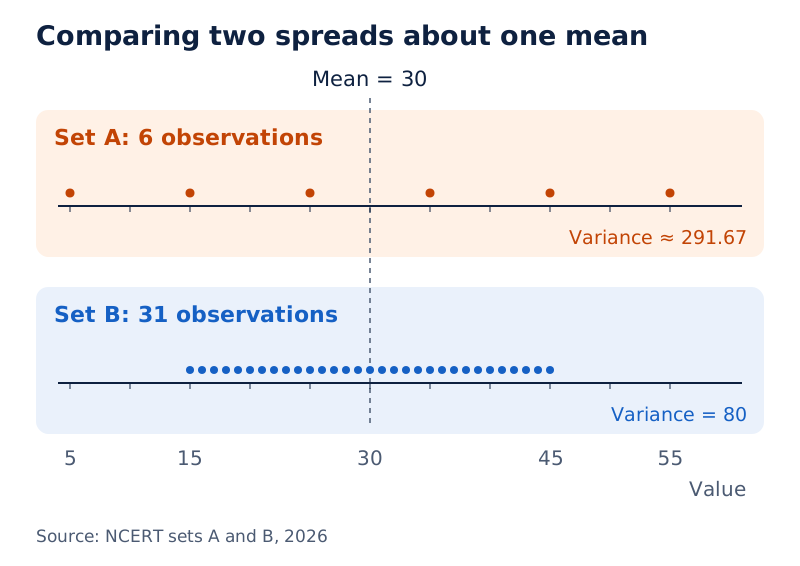
The first number line shows six widely separated dots from $5$ to $55$. The second shows closely spaced dots from $15$ to $45$. Both mark the mean at $30$.

See Figs. 13.5 and 13.6 in your NCERT textbook

What distinguishes variance from standard deviation?

Definition: Variance, denoted by $\sigma^2$, is the mean of the squared deviations from the mean. Standard deviation, denoted by $\sigma$, is the non-negative square root of variance: $$\sigma^2=\frac{1}{n}\sum_{i=1}^{n}(x_i-\bar{x})^2,\qquad\sigma=\sqrt{\frac{1}{n}\sum_{i=1}^{n}(x_i-\bar{x})^2}.$$

Variance has squared units, unlike the observations and their mean. Taking the square root gives standard deviation in the original units. If the squared-deviation sum is zero, each deviation is zero, so every observation equals the mean and there is no dispersion.

How are variance and standard deviation calculated directly?

The direct method begins with the arithmetic mean. Subtract this mean from each value, square each deviation, add the squares, and divide by the number of observations. Take the square root only after completing the variance calculation.

For a frequency distribution, repeated values must contribute repeatedly. This gives $\sigma^2=\frac{1}{N}\sum_{i=1}^{n}f_i(x_i-\bar{x})^2$, with standard deviation $\sigma=\sqrt{\sigma^2}$. The frequency multiplies the squared deviation; it is not included inside the square.

How does the method work for individual observations?

Worked example 7. Find variance and standard deviation for $6,8,10,12,14,16,18,20,22,24$.

Answer: There are ten equally weighted observations.

1. Add the observations and calculate their mean: $$\bar{x}=\frac{6+8+10+12+14+16+18+20+22+24}{10}=\frac{150}{10}=15.$$
2. Subtract the mean to obtain $$-9,-7,-5,-3,-1,1,3,5,7,9.$$
3. Square and add the deviations: $$\sum_{i=1}^{10}(x_i-15)^2=81+49+25+9+1+1+9+25+49+81=330.$$
4. Calculate the variance: $$\sigma^2=\frac{330}{10}=33.$$
5. Take its square root: $$\sigma=\sqrt{33}\approx5.74.$$

How does the method work with frequencies?

Worked example 8. Find variance and standard deviation for the values and frequencies below.

Answer: Use the product column to find the mean before filling the deviation columns.

Value $x_i$	Frequency $f_i$	Product $f_ix_i$	Deviation $x_i-14$	Squared deviation	Weighted square
$4$	$3$	$12$	$-10$	$100$	$300$
$8$	$5$	$40$	$-6$	$36$	$180$
$11$	$9$	$99$	$-3$	$9$	$81$
$17$	$5$	$85$	$3$	$9$	$45$
$20$	$4$	$80$	$6$	$36$	$144$
$24$	$3$	$72$	$10$	$100$	$300$
$32$	$1$	$32$	$18$	$324$	$324$

1. Add the frequencies: $N=3+5+9+5+4+3+1=30$.
2. Find the weighted mean: $$\bar{x}=\frac{12+40+99+85+80+72+32}{30}=\frac{420}{30}=14.$$
3. Subtract $14$, square each result and multiply by its frequency. Add the final column: $$\sum_{i=1}^{7}f_i(x_i-14)^2=300+180+81+45+144+300+324=1374.$$
4. Divide by total frequency: $$\sigma^2=\frac{1374}{30}=45.8.$$
5. Take the square root: $$\sigma=\sqrt{45.8}\approx6.77.$$

For continuous grouped data, replace the classes by their midpoints and follow the same frequency procedure. The distinction is in how the values are obtained, not in the subsequent weighting, squaring or averaging operations.

How is the alternative variance formula derived?

When deviations from the mean are awkward to calculate, variance can be obtained from two totals: the sum of frequency-weighted values and the sum of frequency-weighted squares. This alternative formula follows by expanding the square in the direct definition.

Result: Variance is the mean of squares minus the square of the mean

The result for a frequency distribution is $$\sigma^2=\frac{1}{N}\sum_{i=1}^{n}f_ix_i^2-\bar{x}^{\,2}.$$ The first term is an average of squared values. The second is the square of the average value. Their order matters: subtract the second from the first.

Derivation: Expanding the squared deviation

The totals satisfy $\sum_{i=1}^{n}f_i=N$ and $\sum_{i=1}^{n}f_ix_i=N\bar{x}$.

1. Begin with the definition: $$\sigma^2=\frac{1}{N}\sum_{i=1}^{n}f_i(x_i-\bar{x})^2.$$
2. Expand the square inside the sum: $$\sigma^2=\frac{1}{N}\sum_{i=1}^{n}f_i(x_i^2-2x_i\bar{x}+\bar{x}^{\,2}).$$
3. Separate the sums, treating the mean as constant: $$\sigma^2=\frac{1}{N}\left[\sum_{i=1}^{n}f_ix_i^2-2\bar{x}\sum_{i=1}^{n}f_ix_i+\bar{x}^{\,2}\sum_{i=1}^{n}f_i\right].$$
4. Substitute the two totals: $$\sigma^2=\frac{1}{N}\left[\sum_{i=1}^{n}f_ix_i^2-2N\bar{x}^{\,2}+N\bar{x}^{\,2}\right].$$
5. Combine like terms: $$\sigma^2=\frac{1}{N}\sum_{i=1}^{n}f_ix_i^2-\bar{x}^{\,2}.$$

Standard deviation is therefore $$\sigma=\sqrt{\frac{1}{N}\sum_{i=1}^{n}f_ix_i^2-\left(\frac{1}{N}\sum_{i=1}^{n}f_ix_i\right)^2}.$$

Note: The expression $f_ix_i^2$ means frequency multiplied by the square of the value. It does not mean $(f_ix_i)^2$. In ungrouped data, each observation has unit frequency, so replace the weighted totals by ordinary sums and use the observation count.

The direct and alternative formulas calculate the same variance. One organises the arithmetic around deviations; the other organises it around original values and their squares. This second arrangement is also useful when reconstructing totals from a known mean and standard deviation.

How does the step-deviation method simplify grouped calculations?

The step-deviation method makes large values easier to handle by shifting the origin and reducing the scale. Let $A$ be an assumed mean, $h$ a positive common scale factor, and $y_i$ the transformed value corresponding to $x_i$. Define $y_i=(x_i-A)/h$.

For equally spaced class intervals, their width provides a convenient scale factor. Choose an assumed mean near the middle of the values so that the transformed numbers are small. The frequencies remain attached to the same observations or class midpoints throughout.

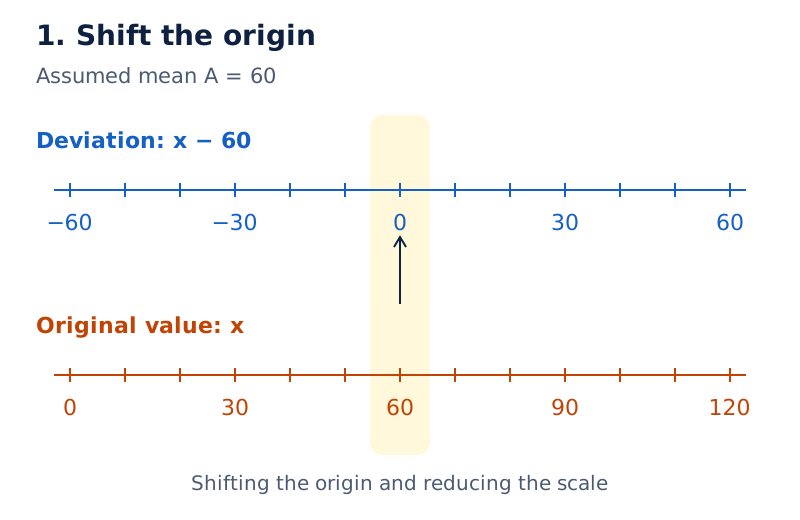
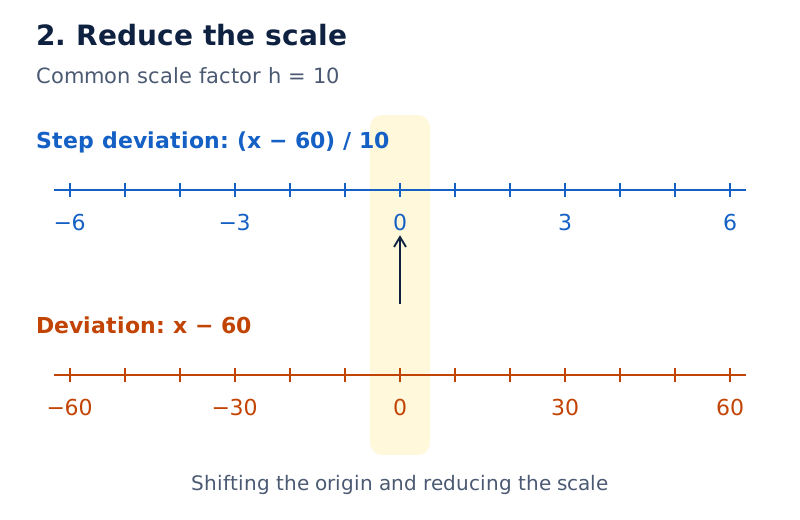
An assumed mean is marked at $60$. The deviation scale places zero above it, with negative values to the left and positive values to the right. The additional step-deviation scale labels these positions from $-6$ to $6$.

See Figs. 13.3 and 13.4 in your NCERT textbook

Derivation: Returning from transformed values

Let $\bar{y}$ be the frequency-weighted mean of the transformed values, and let $\sigma_y^2$ be their variance. Write $\sigma_x^2$ for the variance of the original values and $\sigma_x$ for their standard deviation.

1. Rearrange the transformation: $$x_i=A+hy_i.$$
2. Take weighted means: $$\bar{x}=\frac{1}{N}\sum_{i=1}^{n}f_i(A+hy_i)=A+h\bar{y}.$$
3. Subtract the corresponding means: $$x_i-\bar{x}=A+hy_i-(A+h\bar{y})=h(y_i-\bar{y}).$$
4. Square and average: $$\sigma_x^2=\frac{1}{N}\sum_{i=1}^{n}f_ih^2(y_i-\bar{y})^2=h^2\sigma_y^2.$$

The shortcut formulas are $$\bar{x}=A+h\frac{\sum_{i=1}^{n}f_iy_i}{N},\qquad\sigma_x^2=h^2\left[\frac{\sum_{i=1}^{n}f_iy_i^2}{N}-\left(\frac{\sum_{i=1}^{n}f_iy_i}{N}\right)^2\right].$$

How is the shortcut applied to a full distribution?

Worked example 9. Find the mean, variance and standard deviation of the distribution below using step deviations.

Answer: Take $A=65$ and $h=10$, so $y_i=(x_i-65)/10$.

Class	Frequency $f_i$	Midpoint $x_i$	Step deviation $y_i$	Square $y_i^2$	Product $f_iy_i$	Weighted square $f_iy_i^2$
30 to 40	$3$	$35$	$-3$	$9$	$-9$	$27$
40 to 50	$7$	$45$	$-2$	$4$	$-14$	$28$
50 to 60	$12$	$55$	$-1$	$1$	$-12$	$12$
60 to 70	$15$	$65$	$0$	$0$	$0$	$0$
70 to 80	$8$	$75$	$1$	$1$	$8$	$8$
80 to 90	$3$	$85$	$2$	$4$	$6$	$12$
90 to 100	$2$	$95$	$3$	$9$	$6$	$18$

1. Compute each midpoint, transform it, and square the transformed value as shown. Add frequencies: $N=3+7+12+15+8+3+2=50$.
2. Add the transformed products: $$\sum_{i=1}^{7}f_iy_i=-9-14-12+0+8+6+6=-15,\qquad\sum_{i=1}^{7}f_iy_i^2=27+28+12+0+8+12+18=105.$$
3. Return to the original mean: $$\bar{x}=65+10\left(\frac{-15}{50}\right)=65-3=62.$$
4. Calculate variance with the squared scale factor: $$\sigma_x^2=10^2\left[\frac{105}{50}-\left(\frac{-15}{50}\right)^2\right]=100(2.1-0.09)=201.$$
5. Take the square root: $$\sigma_x=\sqrt{201}\approx14.18.$$

Step deviations can also simplify the mean used in a mean-deviation calculation. Once that mean has been found, calculate the absolute deviations of the original values from it. The remaining mean-deviation procedure is unchanged.

How do changes of origin and scale affect variance?

A change of origin adds the same constant to every observation. A change of scale multiplies every observation by the same constant. These operations affect deviations differently, so their effects on variance must be distinguished.

Property: Adding a constant leaves variance unchanged

Here $a$ denotes a constant added to every observation, $y_i$ the resulting observation, and $\bar{y}$ its mean. The symbols $\sigma_x^2$ and $\sigma_y^2$ denote the original and resulting variances.

1. Write the new observations: $$y_i=x_i+a.$$
2. Average them: $$\bar{y}=\frac{1}{n}\sum_{i=1}^{n}(x_i+a)=\bar{x}+a.$$
3. Subtract the new mean: $$y_i-\bar{y}=(x_i+a)-(\bar{x}+a)=x_i-\bar{x}.$$
4. Square and average: $$\sigma_y^2=\frac{1}{n}\sum_{i=1}^{n}(y_i-\bar{y})^2=\frac{1}{n}\sum_{i=1}^{n}(x_i-\bar{x})^2=\sigma_x^2.$$

The constant cancels from each deviation. Adding or subtracting a fixed number moves the observations and their mean together, leaving their spread about the mean unchanged.

Property: Multiplication changes variance by the square of the multiplier

Let $k$ denote the constant multiplier. Use $y_i$ for the resulting observations in this separate transformation.

1. Write the multiplication: $$y_i=kx_i.$$
2. Take the new mean: $$\bar{y}=\frac{1}{n}\sum_{i=1}^{n}kx_i=k\bar{x}.$$
3. Calculate each deviation: $$y_i-\bar{y}=k(x_i-\bar{x}).$$
4. Square and average: $$\sigma_y^2=\frac{1}{n}\sum_{i=1}^{n}k^2(x_i-\bar{x})^2=k^2\sigma_x^2.$$

Worked example 10. The variance of twenty observations is $5$. Find the new variance when every observation is multiplied by $2$.

Answer: Apply the multiplier to deviations before squaring them.

1. The original squared-deviation total is $$\sum_{i=1}^{20}(x_i-\bar{x})^2=20\times5=100.$$
2. The new mean doubles, so each new deviation also doubles: $$y_i-\bar{y}=2(x_i-\bar{x}).$$
3. The squared-deviation total becomes $2^2\times100=400$.
4. The count is unchanged, giving $$\sigma_y^2=\frac{400}{20}=20.$$

How can missing or incorrect observations be recovered?

A known mean determines the sum of observations. A known variance, together with that mean, determines their sum of squares. These two pieces of information can be used to find missing values or repair calculations based on an incorrectly recorded value.

The useful rearrangements are $\sum_{i=1}^{n}x_i=n\bar{x}$ and $\sum_{i=1}^{n}x_i^2=n(\sigma^2+\bar{x}^{\,2})$. Keep the ordinary sum separate from the squared sum: a correction to one cannot simply be copied into the other.

How are two unknown observations found?

Worked example 11. Five observations have mean $4.4$ and variance $8.24$. Three observations are $1,2,6$. Find the remaining two.

Answer: Let $u$ and $v$ denote the two unknown observations.

1. Use the mean to recover their sum: $$1+2+6+u+v=5\times4.4=22,\qquad u+v=13.$$
2. Use the variance to recover the squared sum: $$1^2+2^2+6^2+u^2+v^2=5(8.24+4.4^2)=138.$$ Hence $u^2+v^2=138-41=97$.
3. Square the sum and subtract the sum of squares: $$2uv=(u+v)^2-(u^2+v^2)=169-97=72.$$
4. Find the squared difference: $$(u-v)^2=u^2+v^2-2uv=97-72=25,\qquad u-v=\pm5.$$
5. Combine the sum and difference: $$\{u,v\}=\left\{\frac{13+5}{2},\frac{13-5}{2}\right\}=\{9,4\}.$$ The unknown observations are $4$ and $9$, in either order.
6. Check the recovered values: $$\bar{x}=\frac{1+2+6+4+9}{5}=4.4,\qquad\sigma^2=\frac{1+4+36+16+81}{5}-4.4^2=8.24.$$

How is an incorrect recorded value replaced?

Worked example 12. The mean and standard deviation of one hundred observations were calculated as $40$ and $5.1$. One value was wrongly recorded as $50$ instead of $40$. Find the correct mean and standard deviation.

Answer: Recover both totals, replace the wrong contribution, and recalculate.

1. Recover the incorrect sum: $$\text{Incorrect sum}=100\times40=4000.$$
2. Replace the incorrect value and calculate the corrected mean: $$\text{Correct sum}=4000-50+40=3990,\qquad\text{correct mean}=\frac{3990}{100}=39.9.$$
3. Recover the incorrect squared sum from the incorrect variance and mean: $$\text{Incorrect squared sum}=100(5.1^2+40^2)=100(26.01+1600)=162601.$$
4. Replace the squared contribution: $$\text{Correct squared sum}=162601-50^2+40^2=162601-2500+1600=161701.$$
5. Use the corrected mean to find the corrected variance: $$\text{Correct variance}=\frac{161701}{100}-39.9^2=1617.01-1592.01=25.$$
6. Take its square root: $$\text{Correct standard deviation}=\sqrt{25}=5.$$

Replacement preserves the observation count. The sum changes by removing the wrong value and adding the correct one; the squared sum changes by removing and adding their squares. The final variance must use the corrected mean as well as the corrected squared sum.

Glossary

• Central tendency — A representative central value, such as the mean, median or mode, around which observations are considered.
• Dispersion — The scatter or variability of observations, describing how spread out or closely grouped they are.
• Range — The difference between the maximum and minimum values in a set of observations.
• Deviation — The difference obtained by subtracting a chosen central or fixed value from an observation.
• Absolute deviation — The distance of an observation from a chosen value, with any negative sign removed.
• Mean deviation — The arithmetic mean of absolute deviations from a specified central value, commonly the mean or median.
• Frequency — The number of occurrences of an observation value, or the number belonging to a class.
• Cumulative frequency — The running total of frequencies up to a particular value or class in ordered data.
• Class midpoint — The value halfway between the limits of a class, used to represent its observations in calculations.
• Median class — The class interval containing the median, located using cumulative frequencies and half the total frequency.
• Variance — The arithmetic mean of squared deviations of observations from their mean, with frequencies included where necessary.
• Standard deviation — The non-negative square root of variance, expressing dispersion in the same units as the observations.
• Assumed mean — A convenient reference value used to simplify calculations by shifting the origin of the observations.
• Step deviation — A deviation from an assumed mean divided by a common factor to simplify numerical calculations.

Common errors and misconceptions

• Misconception: Equal means imply equally scattered observations. Correct: The two batsmen have the same mean and median but different ranges; central tendency does not completely describe variability.
• Misconception: Averaging signed deviations from the mean measures spread. Correct: Their sum is zero. Mean deviation uses absolute values, while variance uses squared deviations.
• Misconception: A discrete median is a cumulative frequency. Correct: Cumulative frequencies locate the central observation or observations; use their values to obtain the median.
• Misconception: Frequency calculations should be divided by the number of rows. Correct: Divide weighted totals by total frequency, because the rows represent repeated observations.
• Misconception: The median of a grouped distribution is automatically its median-class midpoint. Correct: Apply the grouped median formula using the preceding cumulative frequency and the median-class parameters.
• Misconception: Squaring a weighted value gives the required weighted square. Correct: Use $f_ix_i^2$, not $(f_ix_i)^2$; frequency counts how often the squared value contributes.
• Misconception: Multiplying every observation by a constant multiplies variance by that same constant. Correct: Variance changes by the square of the multiplier; adding a constant leaves it unchanged.
• Misconception: Correcting the ordinary sum is enough to repair standard deviation. Correct: Correct the squared sum too, and calculate variance using the corrected mean.

Exam-style questions with model answers

Q1. Define range and explain why it does not fully describe dispersion about a central value. [2 marks]

1. Range is the difference between the maximum and minimum observations: $\text{Range}=\text{maximum value}-\text{minimum value}$.
2. It gives a rough measure of scatter but does not calculate the deviations of observations from a measure of central tendency.

Q2. Find mean deviation about the mean for $6,7,10,12,13,4,8,12$. [4 marks]

1. There are eight observations. Add them and divide by their number to obtain the centre: $\bar{x}=(6+7+10+12+13+4+8+12)/8=72/8=9$.
2. Subtract this mean from each observation in the given order. The signed deviations are $-3,-2,1,3,4,-5,-1,3$.
3. Take absolute values so that negative deviations do not cancel positive ones. Their sum is $3+2+1+3+4+5+1+3=22$.
4. Divide the absolute-deviation total by the number of observations: $\mathrm{MD}(\bar{x})=22/8=2.75$. This is the required mean deviation about the mean.

Q3. Classes 0 to 10, 10 to 20, 20 to 30, 30 to 40, 40 to 50 and 50 to 60 have frequencies $6,7,15,16,4,2$, respectively. Find the median and mean deviation about the median. [5 marks]

1. The total frequency is $N=6+7+15+16+4+2=50$. The cumulative frequencies are $6,13,28,44,48,50$. Since $N/2=25$, the median class is 20 to 30.
2. Its lower limit is $l=20$, preceding cumulative frequency $C=13$, frequency $f=15$, and width $h=10$. Thus $M=20+[(25-13)/15]\times10=28$.
3. Average the two limits of each class to get midpoints $5,15,25,35,45,55$. Their absolute deviations from the median are $23,13,3,7,17,27$, respectively.
4. Multiply these distances by the corresponding class frequencies. The weighted distances are $138,91,45,112,68,54$, giving the total $138+91+45+112+68+54=508$.
5. Divide the weighted absolute-deviation total by the total frequency: $\mathrm{MD}(M)=508/50=10.16$. The required median is $28$, and the mean deviation about that median is $10.16$.

Q4. Find the variance and standard deviation of $6,8,10,12,14,16,18,20,22,24$. [4 marks]

1. Add all ten observations and divide by the count: $\bar{x}=150/10=15$. Use this mean as the centre for every deviation.
2. The deviations are $-9,-7,-5,-3,-1,1,3,5,7,9$. Their squared sum is $81+49+25+9+1+1+9+25+49+81=330$.
3. Variance is the mean of these squared deviations, so divide their sum by the observation count: $\sigma^2=330/10=33$.
4. Standard deviation is the non-negative square root of the variance. Therefore $\sigma=\sqrt{33}\approx5.74$, while the variance remains $33$.

Q5. Prove that adding the same constant $a$ to every observation $x_1,\ldots,x_n$ leaves variance unchanged, where $n$ is the number of observations. [3 marks]

1. Let $y_i=x_i+a$ be the new observations. Denote the original and new means by $\bar{x}$ and $\bar{y}$. Averaging gives $\bar{y}=\frac1n\sum_{i=1}^{n}(x_i+a)=\bar{x}+a$.
2. The new deviation is $y_i-\bar{y}=(x_i+a)-(\bar{x}+a)=x_i-\bar{x}$. The added constant cancels, so each deviation from the corresponding mean is unchanged.
3. Consequently, the new variance is $\frac1n\sum_{i=1}^{n}(y_i-\bar{y})^2=\frac1n\sum_{i=1}^{n}(x_i-\bar{x})^2$. This equals the original variance because both squared deviations and the number of observations remain the same.

Q6. Five observations have mean $4.4$ and variance $8.24$. Three are $1,2,6$. Find the other two. [5 marks]

1. Let $u$ and $v$ be the unknown observations. The total obtained from the mean is $5\times4.4=22$, so $u+v=22-(1+2+6)=13$.
2. Recover the total of squares from the variance: $5(8.24+4.4^2)=138$. Remove the known squared values to get $u^2+v^2=138-(1+4+36)=97$.
3. Square the sum of the two unknowns. Since $(u+v)^2=169$, subtracting their squared sum gives $2uv=169-97=72$.
4. Now $(u-v)^2=u^2+v^2-2uv=97-72=25$, hence $u-v=\pm5$. Together with their sum, this gives $\{u,v\}=\{(13+5)/2,(13-5)/2\}=\{9,4\}$.
5. The remaining observations are therefore $4$ and $9$, in either order. Both original conditions must hold for the recovered observations. Checking all five values gives mean $22/5=4.4$ and variance $138/5-4.4^2=8.24$, agreeing with both conditions.

Q7. One hundred observations gave mean $40$ and standard deviation $5.1$, but one value was recorded as $50$ instead of $40$. Calculate the corrected mean and standard deviation. [6 marks]

1. Use the stated mean and count to reconstruct the incorrect ordinary sum: $100\times40=4000$. The replacement leaves the count at one hundred.
2. Remove the wrongly recorded value and insert the correct value: $4000-50+40=3990$. The corrected mean is therefore $3990/100=39.9$.
3. Square the incorrect standard deviation to get the incorrect variance. The incorrect squared sum is $100(5.1^2+40^2)=100(26.01+1600)=162601$.
4. Correct the squared sum using the squares of the replaced values: $162601-50^2+40^2=162601-2500+1600=161701$.
5. Use both corrected quantities in the variance formula: $161701/100-39.9^2=1617.01-1592.01=25$. The old mean must no longer be used.
6. Take the non-negative square root of this corrected variance: $\sqrt{25}=5$. Thus the corrected mean is $39.9$ and corrected standard deviation is $5$.

Key takeaways

• Measures of central tendency locate a centre; measures of dispersion describe how widely the observations are scattered around it.
• Range uses the largest and smallest observations, whereas mean deviation and standard deviation use deviations from a central value.
• Mean deviation averages absolute deviations, so choose the required mean or median before calculating distances.
• In frequency distributions, multiply each contribution by its frequency and divide the total by the total frequency.
• For continuous grouped data, represent each class by its midpoint when calculating the mean and measures of dispersion.
• Variance averages squared deviations from the mean; standard deviation takes its square root to restore the original units.
• Step deviations simplify arithmetic by shifting the origin and reducing the scale, with variance requiring the squared scale factor.
• Adding a constant leaves variance unchanged, while multiplication changes variance by the square of the multiplier.
• To correct standard deviation after replacing an observation, repair both the ordinary sum and the sum of squares.

Test yourself

Why can two data sets have the same mean but different dispersion?

The mean locates their centre, but observations can be tightly clustered or widely scattered around that same centre.

Why are absolute values used in mean deviation?

They measure distances and prevent positive and negative deviations from cancelling when the deviations are added.

For an even number of ordered observations, how is the median found?

Average the observations in the two central positions, $n/2$ and $n/2+1$, where $n$ is the observation count.

Which cumulative frequency is used in the grouped median formula?

Use the cumulative frequency of the class immediately preceding the median class, not that of the median class itself.

What does zero variance tell you about the observations?

Every squared deviation is zero, so every observation equals the mean and there is no dispersion.

Why is standard deviation expressed in the original units?

Variance squares the deviations and their units; taking its square root restores the units of the original observations.

If variance is $5$ and every observation is doubled, what is the new variance?

The new variance is $2^2\times5=20$, because variance changes by the square of the multiplier.

When an incorrect observation is replaced, does the denominator change?

No. Replacement keeps the observation count unchanged, but both the ordinary sum and squared sum must be corrected.