
Spreadsheet | CBSE Class 12 Accountancy Notes
On this page

This note covers spreadsheet structure, cell references, formulas and functions, logical tests, lookup and financial functions, data entry and validation, formatting, printing, data tables, PivotTable reports and spreadsheet error messages.
What is a spreadsheet, and how is a workbook organised?
Definition: A spreadsheet, also called a worksheet, arranges information in horizontal rows and vertical columns. It is used to record, calculate and compare numerical or financial data.
A spreadsheet application is a computer program for entering and processing data. Microsoft Excel is one such application. The interface and command paths used here are those of Excel 2007, with its Ribbon of tabs and Office Button.
A workbook is an Excel file containing worksheets. In this interface, a new workbook has three sheets by default: Sheet 1, Sheet 2 and Sheet 3. Additional worksheets can be inserted, and sheet names can be changed through the Rename option.
What makes a worksheet or cell active?
The active worksheet is the sheet available for current operations. Only one worksheet is active at a time, and its name appears in bold on the sheet tab. A cell is the intersection of a row and column; the active cell is the currently selected cell.
A cell address identifies a cell by its column letter followed by its row number. A1 is at column A and row 1; G8 is at column G and row 8. The pointer starts at A1 when Excel opens.
The Ribbon groups commands under tabs. The Office Button provides operations such as opening an existing workbook, creating a new one, saving and printing. These operations concern the file, while selecting a sheet or cell determines where worksheet operations take place.
| Movement | Key or combination |
|---|---|
| One cell down | Down arrow or Enter |
| One cell right | Right arrow or Tab |
| Beginning of the current row | Home |
| Cell A1 | Ctrl + Home |
| Intersection of the last row and column containing data | Ctrl + End |
How do cell references and named ranges work?
A cell reference identifies a cell or group of cells used by a formula, function or command. A range is a group of cells. A colon, written as :, separates the first and last addresses of a continuous range, including both endpoints.
The range A1:E2 includes the cells between its upper-left and lower-right corners. References allow a calculation to use values already entered elsewhere. When an input value changes, calculations based on that value can be revised without retyping the relationship.
How do relative, absolute and mixed references differ?
| Reference type | Meaning when a formula is copied | Example |
|---|---|---|
| Relative | References adjust to the new location | C4 |
| Absolute | Both column and row remain fixed | $C$4 |
| Mixed, fixed column | Column remains fixed; row can change | $C4 |
| Mixed, fixed row | Row remains fixed; column can change | C$4 |
The dollar sign, $, fixes the part of the reference immediately following it. Its role here is to control a reference when copying; it is separate from its use as a currency symbol in number formatting.
A named range gives a descriptive name to a cell or range. For example, Numbers can represent B1:F1. The formula =SUM(Numbers) then uses the same range as =SUM(B1:F1). SUM is the built-in function that adds its supplied values.
- Select the cells to name, such as B1:F1.
- Open the Formulas tab and choose Define Name.
- Enter Numbers in the Name box and check the range in Refers to.
- Click OK, then use the name in the required formula or through Apply Names.
What the figure shows
Cell references and naming tools
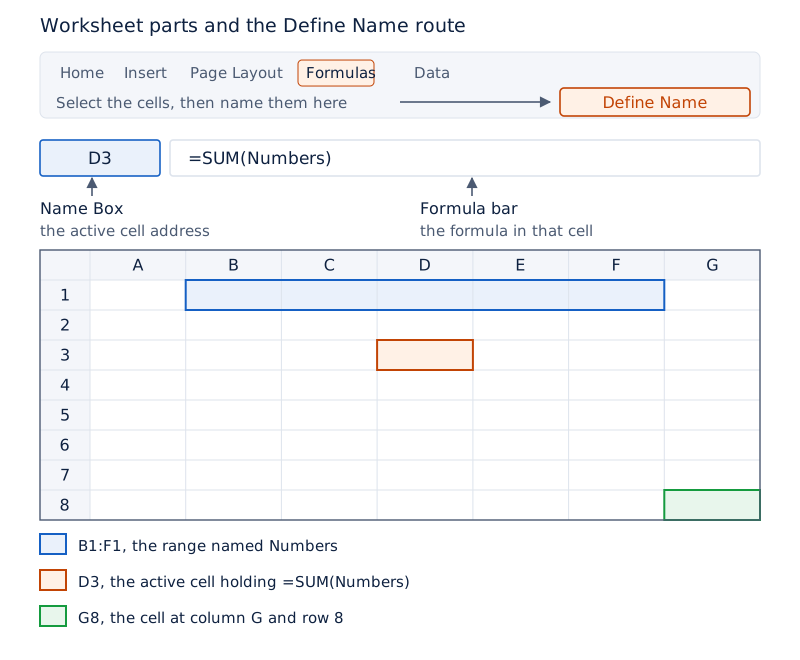
The worksheet screenshot shows lettered columns, numbered rows, a Name Box and a formula bar. Arrows identify the Name Box and formula bar, while Define Name is circled on the Ribbon.
Drawn by One Young India. See Fig. 2.3 in your NCERT textbook
How do basic values, formulas and functions produce results?
A basic value is entered independently. A derived value is calculated from other values through an arithmetic expression or function. An arithmetic expression combines values using mathematical operations; a formula specifies the calculation whose result appears in its cell.
Let Q mean quantity purchased, P mean price per item and V mean the value of the purchase. The relationship is V = Q × P, where × means multiplication. Q and P are basic values; V is derived.
Excel formulas begin with =, the equal sign. Within spreadsheet formulas, + means addition, - means subtraction, * means multiplication, / means division and ^ means raising to a power. Brackets group operations that must be performed together.
In what order are operations performed?
- Carry out operations within brackets first.
- Evaluate exponents, which specify powers.
- Perform multiplication and division with equal priority, working from left to right.
- Perform addition and subtraction with equal priority, working from left to right.
A function is a built-in calculation identified by a special name. Its arguments are the values, references or other inputs supplied inside brackets. To understand a function, identify its name, purpose, required arguments and result.
Worked example 1. Cells D1, E1, F1 and G1 contain 4, 3, 2 and 8 respectively. Find their total using SUM.
Answer: Enter =SUM(D1:G1). The calculation is 4 + 3 + 2 + 8 = 17. The result appears in the cell containing the function; D1:G1 identifies the input range.
What the figure shows
Adding a range with SUM
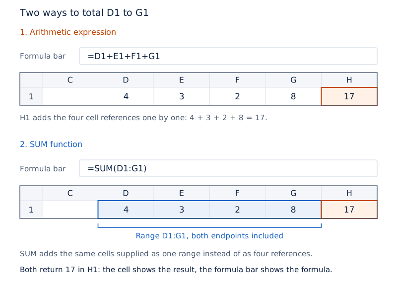
The screenshots show the values 4, 3, 2 and 8 across D1:G1, the formula =SUM(D1:G1), and the result 17. Arrows distinguish an arithmetic sum from the SUM function.
Drawn by One Young India. See Figs. 2.9(a) and 2.9(b) in your NCERT textbook
The formula bar displays the selected cell's formula, while the cell displays its calculated result. A formula often contains references to other cells. A worksheet without formulas can still organise information as a list, timetable or other arrangement of data.
To retain a calculated result without its formula, select the cell, copy it, open Paste Special and choose Values. This replaces the formula with its current result. The retained value will no longer be recalculated by that formula when earlier inputs change.
How are totals, averages, rounding and text functions used?
SUM returns a total, AVERAGE returns the arithmetic mean, and COUNT counts numeric entries. The arithmetic mean is the total of the numbers divided by their count. AutoSum provides access to these and other series-based functions, including MIN and MAX for minimum and maximum values.
COUNTA can count entries such as text, logical values and error values. A logical value is TRUE or FALSE. COUNTIF(range, criteria) counts cells meeting a condition: range identifies the cells to examine, and criteria specifies the condition.
SUMIF(range, criteria, sum_range) adds values conditionally. Here range contains the cells to evaluate, criteria states which entries qualify, and sum_range contains the corresponding values to add. A condition can be a number, text or an expression comparing values.
How does rounding differ from changing the display?
ROUND(number, num_digits) rounds a supplied number to the precision specified by num_digits. A positive num_digits specifies decimal places; zero rounds to an integer, meaning a whole number; a negative value rounds to the left of the decimal point.
Worked example 2. Round 3.14159 to three decimal places using ROUNDUP and ROUNDDOWN.
Answer: =ROUNDUP(3.14159,3) gives 3.142 because ROUNDUP rounds away from zero. =ROUNDDOWN(3.14159,3) gives 3.141 because ROUNDDOWN rounds towards zero. The second argument, 3, specifies three decimal places.
TEXT(value, format_text) converts a numeric value into text in a specified format. Value is the number or reference to convert; format_text is the format enclosed in quotation marks. For L1 containing 23.5, =TEXT(L1,"Rs. 0.00") displays Rs. 23.50, where Rs. denotes rupees.
CONCATENATE(text1, text2,...) joins text items into one text string, meaning a sequence of characters. The arguments text1 and text2 represent items to join; the dots indicate further items. It can combine an employee's first name, middle name and surname.
ROWS(array) and COLUMNS(array) count rows and columns respectively. Here an array is a group of values arranged in rows and columns, or a reference to such a group. These functions describe its dimensions rather than adding its contents.
How do IF, AND and OR test conditions?
IF returns one result when a condition is TRUE and another when it is FALSE. Its form is =IF(logical_test, value_if_true, value_if_false). The logical_test is the condition; value_if_true and value_if_false specify the results for the two possible outcomes.
A logical operator compares values. The symbols <, >, =, <=, >= and <> mean less than, greater than, equal to, less than or equal to, greater than or equal to, and not equal to respectively.
In =IF(A1<20,"Yes","No"), A1 is the cell being tested. The result is Yes when its value is below 20, and No otherwise. Quotation marks enclose the text results. The returned result can also be a number, expression or referenced value.
How can several conditions be combined?
A nested IF places an IF function inside another IF. This permits further tests when a branch of the first test is followed. The function =IF(E2<96,IF(E2<91,IF(E2<55,"Fail","C Grade"),"B Grade"),"A Grade") uses the test marks in E2 to choose a result.
AND returns TRUE when all its arguments are TRUE, and FALSE if one or more are FALSE. OR returns TRUE when any argument is TRUE, and FALSE when all are FALSE. Both can supply the logical_test argument within IF.
Worked example 3. Cell A2 contains 50 and A3 contains 104. Test whether each number is greater than 1 and less than 100.
Answer: =AND(A2>1,A2<100) returns TRUE because 50 meets both conditions. =IF(AND(A3>1,A3<100),A3,"The value is out of range.") returns the message because 104 fails the second condition.
What-if analysis examines how changes in inputs affect results. For interest calculations, define PA as principal amount, the original sum; MA as maturity amount, the final amount payable; and CI as compound interest, interest calculated with compounding, meaning that accumulated interest is included in subsequent interest calculations. Then CI = MA - PA. Changing inputs such as interest rate allows alternative outcomes to be compared.
How do lookup functions retrieve information?
LOOKUP searches for a value and retrieves a related result. Its vector form uses =LOOKUP(lookup_value, lookup_vector, result_vector). A vector is a single row or column. The lookup_value is the item sought; lookup_vector is searched; result_vector supplies the corresponding result.
The two vectors must have the same size, and the lookup vector must be in ascending order. If an exact match is absent, LOOKUP uses the largest value less than or equal to the requested value. A request below the smallest value gives #N/A, meaning a value is unavailable.
| Cell in column A | Frequency | Colour in column B |
|---|---|---|
| A2 | 4.14 | red |
| A3 | 4.19 | orange |
| A4 | 5.17 | yellow |
| A5 | 5.77 | green |
| A6 | 6.39 | blue |
Worked example 4. Use the frequency and colour data above, stored in A2:B6, to retrieve the colour for a lookup value of 7.66.
Answer: =LOOKUP(7.66,A2:A6,B2:B6) returns blue. There is no exact match for 7.66. The largest listed frequency below it is 6.39, whose corresponding colour is blue.
How do vertical and horizontal lookup differ?
VLOOKUP, or vertical lookup, searches the first column of a table and returns a value from another column in the same row. Its form is =VLOOKUP(lookup_value, table_array, col_index_num, range_lookup).
Here table_array is the table range, col_index_num is the number of the return column within that table, and range_lookup specifies matching. FALSE requires an exact match. TRUE or an omitted argument permits an approximate match and requires ascending order in the first column.
HLOOKUP, or horizontal lookup, searches the first row and returns a value from another row in the same column. Its corresponding argument row_index_num identifies the return row. Absolute references keep a lookup table fixed when formulas are copied.
In the quarterly budget application, D4 contains the budget and E4 contains the amount spent. The amount still pending is Pending = D4 - E4. The lookup first retrieves the appropriate quarter's budget; subtraction then calculates the pending amount.
What do date and financial functions calculate?
TODAY() returns the current date, while NOW() includes the current time. Excel represents dates with serial numbers and times with fractions of a day. DAY, MONTH and YEAR extract the corresponding parts of a supplied date.
DATEVALUE(date_text) converts a date written as text into a serial number; date_text is the quoted date text. Dates can therefore be used in calculations. The date display format depends on the selected country-specific format.
Which arguments recur in financial functions?
An annuity is a series of constant cash payments over a continuous period. In financial functions, rate means interest rate per period, nper means number of payment periods, and pmt means payment each period. Present value, pv, is what future payments are worth now.
Future value, fv, is the cash balance after the final payment. The argument type specifies payment timing: 0 means the end of a period and 1 means the beginning. Keep the units of rate and nper consistent, such as monthly interest with monthly payments.
| Function | Purpose |
|---|---|
| PV(rate,nper,pmt,fv,type) | Finds present value |
| FV(rate,nper,pmt,pv,type) | Finds future value with constant periodic payments and a constant interest rate |
| PMT(rate,nper,pv,fv,type) | Finds the periodic payment with equal payments and a constant interest rate |
| RATE(nper,pmt,pv,fv,type,guess) | Finds interest rate per period; guess is an initial estimate of that rate |
Payment amounts typically include principal and interest but no other fees or taxes. The pv, fv and pmt arguments can be positive or negative depending on whether money is received or paid. PMT is often used for fixed-interest mortgage loan payments, meaning payments on a loan secured against property.
CUMIPMT calculates cumulative interest paid between specified starting and ending periods. ACCRINT calculates accrued interest, meaning accumulated interest, for a security, a financial instrument, paying periodic interest. NPV, net present value, discounts a sequence of future payments and receipts, meaning it converts them to their present worth.
For NPV, the cash flows must be equally spaced and occur at each period's end. Their order matters. Unlike the variable cash flows used by NPV, the cash flows for PV must remain constant throughout the investment.
How can data be entered, validated and edited efficiently?
A label is descriptive text, such as a heading or name, rather than a quantity for mathematical operations. Data can be typed directly, filled as a series, copied or imported. Numbers are right aligned by default, while text is left aligned.
The fill handle is the small square at the lower-right corner of a selection. Dragging it can continue a pattern. For a sequence starting at 10 with a step of 10 and stopping at 100, Fill Series can populate A1:A10.
A CSV, or Comma Separated Values, text file separates successive entries with commas. One line corresponds to a spreadsheet row. In Excel 2007, Data, Get External Data and From Text provide the route for importing text data.
How does validation restrict entries?
Data validation defines restrictions on entries. A drop-down list restricts selection to listed items. Limits can also be set for whole numbers, decimals, dates, time or text length. An input message explains the expected entry; an error alert responds to invalid data.
- Prepare the permitted department names and define their range as DEPT.
- Select the cells that will receive department entries.
- Open Data Validation from the Data tab and choose List in the Settings tab.
- Enter =DEPT as the Source and use the in-cell drop-down option.
- Set an Input Message and the required Error Alert for the selected cells.
A custom validation formula makes an entry valid when it returns TRUE and invalid when it returns FALSE. It can help prevent duplicate codes, restrict a total to a budget, or reject specified days of the week.
A data form displays one complete record at a time. A record is one row of related data. The form uses column headings as labels and can add, locate, change or delete records. It displays formula results but cannot change formulas through the form.
In Excel 2007, add Form to the Quick Access Toolbar through More Commands, All Commands and Add. Enter headings in the first worksheet row before using it. A data form can display up to 32 columns in a single dialogue box.
How does formatting make a spreadsheet easier to read?
Formatting controls presentation. Number formatting can show currency signs, percentages, decimal places, dates or time. It changes the displayed value rather than the cell's underlying contents. A formatted number and a number converted into text with TEXT therefore serve different purposes.
Use Format Cells to choose a category and its options. Currency formatting allows the currency symbol, decimal places and negative-number presentation to be selected. Custom formatting allows an existing format to be adapted by adding or removing characters.
What does conditional formatting do?
Conditional formatting changes appearance according to a condition. When the condition is true, the specified formatting applies; when false, that formatting does not apply. It helps highlight unusual values or important ranges through data bars, colour scales and icon sets.
A colour scale uses different shades to show differences in values. Select the range, open Home, choose Conditional Formatting in the Styles group, and select Colour Scales. Manage Rules allows a rule to be created or edited.
Text formatting includes the font, meaning the lettering style, its size, colour and alignment. Alignment sets the position of content within a cell. Borders and background fills can distinguish headings and groups. Format Painter copies formatting to another cell or range.
Merged cells combine adjacent cells into one larger cell. Select the cells and use Merge and Centre in the Home tab's Alignment group. To split a merged cell, select it and click Merge and Centre again; the contents appear in the upper-left cell.
Format as Table applies a predefined table style to a selected range. Styles are grouped as Light, Medium or Dark. Existing tables can use Table Styles on the Design tab, and custom styles can be created when the predefined choices do not meet requirements.
How are print areas, headers and output reports prepared?
An output report presents processed worksheet information. Excel can print all or part of a worksheet, several worksheets or workbooks, a table, or a workbook to a file. Print Preview lets the user inspect the intended printout before printing.
A header is text printed at the top of each page; a footer appears at the bottom. They can contain descriptive titles, dates or page numbers. In Page Layout view, use Insert, Text and Header and Footer, then enter the required text.
How is a print area defined?
The print area is the range selected for printing. Excel keeps it until it is cleared or replaced. Defining this area identifies the report cells that should appear in the printout rather than relying on all data in the active sheet.
- Select the range to print, such as A1:H10.
- Open the Page Layout tab.
- In Page Setup, choose Print Area and Set Print Area.
- To include another range, select it and choose Add to Print Area.
- To remove the stored selection, use Clear Print Area.
Alternatively, open the Page Setup dialogue box, select the Sheet tab and enter the range in the Print Area box. The selection controls can temporarily collapse the dialogue box while the range is selected on the worksheet.
For a manually selected range, open Print with Ctrl + P and choose Selection under Print what. To select several non-contiguous ranges, meaning ranges that are not adjacent, hold Ctrl while selecting additional ranges. These selected ranges print on separate pages.
How do data tables and PivotTables support analysis?
A data table shows results obtained by substituting different inputs into formulas. A one-variable data table varies one input cell. A two-variable data table uses one formula referring to two input cells and two lists of possible inputs.
For a column-oriented one-variable table, the inputs run down a column. Place the formula above the first input and one column to its right. Select the table range, choose Data, What-if Analysis and Data Table, then specify the Column input cell.
How does a PivotTable summarise records?
A PivotTable creates a cross-tabulation, meaning a summary arranged by categories across rows and columns. Headings can be moved to give different views. A PivotTable report often provides enhanced layout and improved readability, with suitable calculations and levels of detail.
The vegetable-consumption example uses Carrot, Onions and Potatoes, three days, and four cities. Its fields include actual consumption and quota, meaning the fixed consumption allocation. The worksheet calculates the field labelled surplus as Surplus = Actual - Quota.
- Select the source data range A1:E37.
- Choose Insert, then PivotTable in the Tables group.
- Confirm the data location and choose a report destination, such as G19 on an existing worksheet.
- Click OK to display the blank PivotTable and field list.
- Place Day in Report Filter, Vegetable in Column Labels, City in Row Labels and Sum of Actual in Values.
A report filter selects which data the report displays. Row and column labels organise categories, while Values contains the summarised figures. Changing these placements changes the summary view, allowing related totals to be compared in different ways.
What the figure shows
Alternative PivotTable layouts
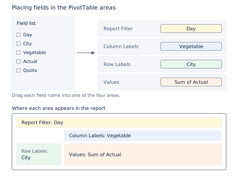
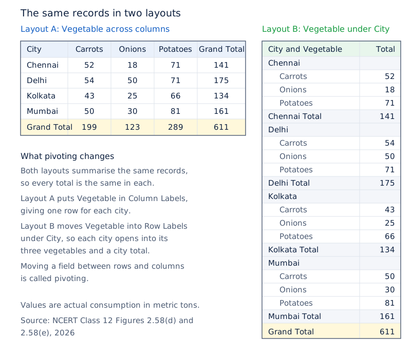
The screenshots show the field list and report areas, followed by a summary with cities in rows and vegetables in columns. Another layout nests vegetables below cities.
Drawn by One Young India. See Figs. 2.58(c), 2.58(d) and 2.58(e) in your NCERT textbook
PivotTables can aggregate, meaning combine, numeric data; create subtotals; expand or collapse detail; and filter, sort or group information. Moving rows to columns or columns to rows is called pivoting. These operations help examine large amounts of data and prepare concise reports.
How should common spreadsheet errors be interpreted?
A spreadsheet displays an error value when it cannot evaluate a formula properly. The message identifies a type of problem, but its cause must be checked. Background error checking can mark a cell with a triangle and provide options through the Error Checking button.
Which message points to which problem?
| Message | Meaning or cause | Check or response |
|---|---|---|
| ##### | Column too narrow, or negative date or time | Check column width and the date or time calculation |
| #DIV/0! | Division by zero, including a blank divisor cell | Check the divisor, meaning the value used to divide |
| #N/A | Required value is unavailable | Check missing data and lookup inputs |
| #NAME? | Excel does not recognise text in a formula | Check the formula text and required functions |
| #NULL! | Specified areas do not intersect | Check the range operator and references |
| #NUM! | Invalid numeric values or an unsuccessful iterative calculation | Check numeric arguments and calculation settings |
| #REF! | Invalid cell reference | Check deleted or overwritten referenced cells |
| #VALUE! | Wrong argument or operand type | Check that the inputs suit the calculation |
An operand is an item on either side of an operator, such as a value or reference. An iterative calculation repeatedly recalculates while seeking a result. RATE can have zero or more solutions, so a result should not be assumed merely because the function was entered.
For a narrow column, AutoFit Column Width or an appropriate display format can help. For an invalid reference created by deleting cells, change the formula or use Undo immediately to restore the cells. Match the remedy to the actual cause.
The formula =IF(B5=0,"",A5/B5) avoids displaying division by zero by returning an empty text string, written as two quotation marks with nothing between them. A5 is the number being divided; B5 is the divisor. Otherwise, the formula performs the division.
Glossary
- Workbook — An Excel file containing a collection of worksheets used to organise information.
- Worksheet — A grid of rows and columns for recording, calculating and comparing data.
- Cell — The intersection of a row and column where data or formulas can be entered.
- Cell reference — An address identifying a cell or group of cells used in a calculation.
- Absolute reference — A reference whose column and row remain fixed when its formula is copied.
- Named range — A descriptive name assigned to cells and usable in place of their references.
- Formula — An instruction specifying the calculation whose result is displayed in its cell.
- Argument — A value, reference or other input supplied to a function for its operation.
- Logical test — A condition evaluated to determine whether its result is TRUE or FALSE.
- Data validation — A feature setting restrictions on the data users enter into selected cells.
- Conditional formatting — Formatting that changes the appearance of selected cells according to a condition.
- PivotTable — An interactive summary whose category headings can be rearranged to show different views.
Common errors and misconceptions
- Misconception: A workbook and worksheet are the same. Correct: A workbook is a file containing worksheets; a worksheet is the grid used for data and calculations.
- Misconception: A reference stays fixed whenever its formula is copied. Correct: Relative references adjust. Dollar signs fix the required row, column or both parts of a reference.
- Misconception: Multiplication must precede division everywhere. Correct: Multiplication and division have equal priority and are evaluated from left to right after brackets and exponents.
- Misconception: OR requires every condition to be TRUE. Correct: OR requires any condition to be TRUE. AND requires all its conditions to be TRUE.
- Misconception: VLOOKUP with FALSE returns an approximate match. Correct: FALSE requires an exact match; an absent exact match gives #N/A.
- Misconception: Number formatting changes the stored contents. Correct: Formatting changes the display. TEXT instead converts a numeric value into a text result.
- Misconception: Every ##### display means division by zero. Correct: Check column width or negative dates and times. Division by zero produces #DIV/0!.
Exam-style questions with model answers
Q1. Distinguish a workbook from an active worksheet. [2 marks]
- A workbook is an Excel file containing a collection of worksheets for organising data.
- The active worksheet is the single sheet currently available for operations; its sheet-tab name appears in bold.
Q2. Explain relative, absolute and mixed cell references, giving the forms C4, $C$4, $C4 and C$4. [3 marks]
- C4 is a relative reference. When a formula containing it is copied to another location, the reference adjusts to that location.
- $C$4 is an absolute reference. The dollar signs fix both column C and row 4 when the formula is copied.
- $C4 fixes the column, while C$4 fixes the row. These are mixed references because one part stays fixed and the other can change.
Q3. Cells D1, E1, F1 and G1 contain 4, 3, 2 and 8 respectively. Write a SUM formula and explain the result and the meaning of D1:G1. [3 marks]
- Enter =SUM(D1:G1) in the cell where the answer is required. The equal sign starts the formula and SUM adds the supplied range.
- D1:G1 is the continuous range from D1 through G1, including both endpoints. The colon identifies all four cells as inputs.
- The answer is 17, calculated as 4 + 3 + 2 + 8. Excel displays that result in the cell containing the function.
Q4. Cell A2 contains 50 and A3 contains 104. Explain AND, evaluate =AND(A2>1,A2<100), state its result if A3 replaces A2, and distinguish OR. [4 marks]
- AND returns TRUE when all its conditions are TRUE, and FALSE if one or more conditions are FALSE.
- For A2, 50 is greater than 1 and less than 100. Both comparisons are TRUE, so the function returns TRUE.
- For A3, 104 is greater than 1 but is not less than 100. The combined AND result is therefore FALSE.
- OR returns TRUE when any condition is TRUE. It returns FALSE only when all its conditions are FALSE.
Q5. A2:A6 contains 4.14, 4.19, 5.17, 5.77 and 6.39, in that order. B2:B6 contains red, orange, yellow, green and blue, respectively. Explain the vector arrangement and find the LOOKUP results for 4.19, 5.00, 7.66 and 0. [5 marks]
- A2:A6 is the ascending lookup vector, while B2:B6 is the result vector. Each contains five cells, and corresponding positions connect a frequency with its colour.
- =LOOKUP(4.19,A2:A6,B2:B6) returns orange because 4.19 is an exact match. The result comes from the same position in the second vector.
- =LOOKUP(5.00,A2:A6,B2:B6) also returns orange. With no exact match, the largest listed frequency less than or equal to 5.00 is 4.19.
- =LOOKUP(7.66,A2:A6,B2:B6) returns blue. The largest available frequency below the lookup value is 6.39, and its corresponding colour is blue.
- =LOOKUP(0,A2:A6,B2:B6) returns #N/A. Zero is below the smallest frequency, 4.14, so there is no qualifying value in the lookup vector.
Q6. A worksheet needs department entries restricted to the named range DEPT. Explain five steps for configuring list validation, an input message and an error alert in Excel 2007. [5 marks]
- Prepare the list of permitted department names and define it as the named range DEPT. This range supplies the values available for selection.
- Select the cells in which department entries will be made. Open the Data tab and choose Data Validation from the Data Tools group.
- In the Settings tab, select List and enter =DEPT in the Source box. Use the in-cell drop-down option for selecting permitted departments.
- Open the Input Message tab and enter a suitable title and message explaining the expected entry. Enable its display when the cell is selected.
- Use the Error Alert tab to set the message shown for invalid entries and the required alert style. Stop prevents an invalid entry.
Q7. Explain six uses of a PivotTable report when analysing a long list of numerical records. [6 marks]
- It summarises large amounts of numerical data into a report, helping the user examine related totals and respond to questions about the data.
- It aggregates numeric values and creates subtotals by categories and subcategories, so the same records can support several levels of summary.
- It allows levels of detail to be expanded or collapsed, helping the user move between overall results and particular areas of interest.
- It permits rows to be moved to columns or columns to rows. This pivoting provides different summary views of the source data.
- It supports filtering, sorting, grouping and conditional formatting, allowing attention to be directed towards a useful subset of the available information.
- It presents concise, attractive and annotated reports for viewing online or printing, with calculations and a layout suited to the required information.
Q8. A formula divides a number by a blank cell. Identify the likely error message and give one correction. [2 marks]
- The likely error is #DIV/0! because a blank cell used as the divisor is treated as zero in this calculation.
- Enter the required non-zero value in the divisor cell, or correct the reference if the formula points to the wrong cell.
Key takeaways
- A workbook contains worksheets, and each worksheet organises data in cells identified by column letters and row numbers.
- Relative references adjust when copied; absolute references stay fixed, while mixed references fix either the row or column.
- Formulas express calculations, while functions provide built-in operations using arguments such as values, ranges and conditions.
- IF selects between outcomes, AND requires every condition to be TRUE, and OR requires any condition to be TRUE.
- Lookup functions connect a search value with related information; the selected matching option determines whether an exact match is required.
- Financial functions require consistent periods for rates and payments, with appropriate signs for money received or paid.
- Validation restricts entries, formatting controls presentation, and print-area settings determine which report cells are printed.
- Data tables compare input alternatives, while PivotTables summarise records and rearrange categories to reveal different views.
Test yourself
What does the colon in A1:E2 mean?
It includes the entire range between the two corner cells, including A1 and E2.
What remains fixed in the reference C$4?
Row 4 remains fixed, while the column can adjust when the formula is copied.
In which direction do ROUNDUP and ROUNDDOWN round numbers relative to zero?
ROUNDUP rounds away from zero; ROUNDDOWN rounds towards zero at the specified precision.
What is the difference between TODAY() and NOW()?
TODAY() returns the current date, whereas NOW() returns the current date and time.
What does type = 1 mean in the financial functions discussed?
It specifies that payments are made at the beginning of each period.
Can a data form change a formula?
No. It displays the formula's result, but the formula cannot be changed through the data form.
How does Paste Special with Values affect a formula?
It replaces the formula with its current calculated value, preventing that formula from recalculating.
What does #REF! indicate?
It indicates an invalid reference, which can result from deleting cells used by a formula.
Write about it
Turn a question from this chapter into a paper.
The Writing Studio has a structure guide, a rubric and citation tools for 15 formats, from essays to research papers. Drafting is free with an account. Learnacy Essential adds feedback from an AI writing coach and submission to The OYI Review.
Learnacy Essential is ₹1,499 for the year. Publication depends on review and is not guaranteed.